Dissecting Reinforcement Learning-Part.8
In the last post I introduced function approximation as a method for representing the utility function in a reinforcement learning setting. The simple approximator we used was based on a linear combination of features and it was quite limited because it could not model complex state spaces (like the XOR gridworld). In this post I will introduce Artificial Neural Networks as non-linear function approximators and I will show you how we can use a neural network to model an utility function. I will start from a basic architecture called Perceptron and then move to the standard feedforward model called Multi Layer Perceptron (MLP). Moreover, as bonus material I will introduce policy gradient methods that are (most of the time) based on neural network policies. I will use pure Numpy to implement the network and the update rule, in this way you will have a transparent code to study. This post is important because it allows understanding the deep models (e.g. Convolutional Neural Networks) used in Deep Reinforcement Learning, that I will introduce in the next post.
The reference for this post is chapter 8 for the Sutton and Barto’s book called “Generalization and Function Approximation”. Recently the second version of the book has been released, you can easily find a pre-print for free on DuckDuckGo. Moreover a good resource is the video-lesson 7 of David Silver’s course. A wider introduction to neural networks is given in the book “Deep Learning” written by Goodfellow, Bengio, and Courville.
I want to start this post with a brief history of neural networks. I will show you how the first neural network had the same limitation of the linear models considered in the previous post. Then I will present the standard neural network known as Multi Layer Perceptron (MLP) and I will show you how we can use it to model any utility function. This post can be heavy compared to the previous ones but I suggest you to study it carefully, because the use of neural networks as function approximators is the scaffolding sustaining modern RL approaches.
The life and death of the Perceptron
In 1957 the American psychologist Frank Rosenblatt presented a report entitled “The Perceptron: a perceiving and recognizing automaton” to the Cornell Aeronautical Laboratory commission in New York. The Perceptron was not a proper software, it was implemented in a custom hardware (as big as a wardrobe), and it could discriminate between two types of marked cards. The first series of cards was marked on the left side, whereas the second series was marked on the right. A grid of 400 photo-cells was able to locate the marks and activate mechanical relays. Adjusting the parameters of the Perceptron was not so easy as today. In pyTorch/Tensorflow we simply define a bunch of variables and then we search for the best combinations. In the hardware implementation the parameters to tune were physical handles (potentiometers) adjusted through electric motors.
For your joy I found the original article of The New York Times describing the official presentation of the Perceptron by Rosenblatt and his staff:
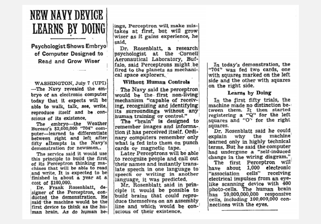
As you have read the power of the Perceptron was a bit overestimated, especially when talking about artificial brains that “would be conscious of their existence” (we could start here a long discussion about what consciousness really is, but it would take another blog series). However, some of the predictions made by Rosenblatt were correct:
“Later perceptrons will be able to recognize people and call out their names and instantly translate speech in one language to speech or writing in another language”
Well, it took several decades but we now have it. What is the Perceptron from a technical point of view? You might be surprised to know that the Perceptron is a linear function approximator like the one described in the previous post. Let’s try to formalise this point. The input to the Rosenblat’s Perceptron were 400 binary photo-cells that we can model as a vector of units \(\boldsymbol{x} = ( x_{1}, x_{2,}, ..., x_{400} )\). The output was given by an electric tension that we can call \(y\). The connection between input and output were a series of wires and potentiometers that we can model through another vector \(\boldsymbol{w}\) containing 400 real values (the resistance of the potentiometers). I said that the Perceptron is a linear system, and exactly like the linear model described in the previous post we can define it as the dot product between two vectors \(\boldsymbol{x}^{T} \boldsymbol{w}\). However, there is an intermediate step: the use of an activation function called \(\phi\) that takes as input the result of the weighted sum and generates the output \(y\):
\[y = \phi \big( \boldsymbol{x}^{T} \boldsymbol{w} \big)\]We can also use an additional bias unit called \(x_{b}\) and its weight \(w_{b}\). We can append the additional input to the vector \(\boldsymbol{x}\), and we can append the additional weight to the vector \(\boldsymbol{w}\). The reason for a bias unit has been extensively discussed in the previous post and I suggest you to give a look if you do not remeber why we need it. The last equation is the final form of the Perceptron. It may be useful to graphically represent the Perceptron as a directed graph where each node is a unit (or neuron) and each edge is a weight (or synapse). Regarding the name convention there is not a clear rule in the community. I personally prefer to use the term unit and weight instead of neuron and synapse to avoid confusion with the biological counterpart.
The following image represent the Rosenblatt’s Perceptron. The 400 photo-cell fires only when a mark is identified on the card. Each photo-cell can be thought as an input of the Perceptron. Here I represented the neurons using a green colour for the active units (state=1), a red colour for the inactive units (state=0), and an orange colour for the units with undefined state. When I say “undefined state” I mean that the output of that unit has not been computed yet. For instance, this is the state of the output unit \(y\) before the weighted sum and the transfer function are applied. In the image you must notice that the bias unit is always active, if you remember the last post, we used this trick in order to add the bias in our model.
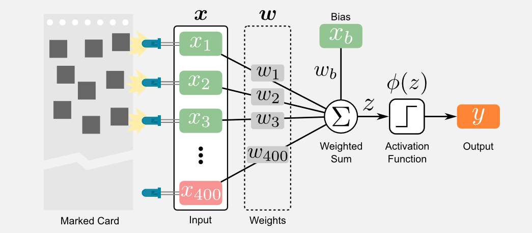
As I told you above, the only difference between the linear approximator and the Perceptron is the activation function \(\phi\). The original perceptron uses a sign function to generate a binary output of type zero/one. The sign function introduce a relevant problem. Using a sign function it is not possible to apply gradient descent because this function is not differentiable. Another important detail I should tell you is that gradient based techniques (such as the backpropagation) were unknown at that time.
How did Rosenblatt train the Perceptron? Here is the cool part, Rosenblatt used a form of Hebbian learning. The psychologist Donald Hebb had published a few years before (1949) the work entitled “The Organization of Behavior” where he explained cognitive processes from the point of view of neural connectivity patterns. The principle is easy to grasp: when two neurons fire at the same time their connection is strengthened. Ronsenblat was inspired by this work when he defined the update rule of the Perceptron. The update rule directly manages the three possible outcomes of the training phase and it is repeated for a certain number of epochs:
- If the output \(y\) is correct, leave the weights \(w\) unchanged
- If the output \(y\) is incorrect (zero instead of one), add the input vector \(x\) to the weight vector \(w\)
- If the output \(y\) is incorrect (one instead of zero), subtract the input vector \(x\) from the weight vector \(w\)
The geometric interpretation of the update rule can help you understand what is going on. I said that \(w\) is a vector, meaning that we can imagine this vector in a three-dimensional space. The starting point of the vector is at the origin of the axes, whereas the end of the vector is at the coordinates specified by its values. The set of all the input vectors can also be considered as a bunch of vectors that occupy part of the same three-dimensional space. What we are doing during the update is moving the weight vector changing its end-coordinates. The optimal position of the vector is inside a cone (with apex in the origin) where the first criterion of the learning rule is always satisfied. Said differently, when the weight vector reach this cone the second and third conditions of the update rule are no more triggered.
Implementing a Perceptron and its update rule in Python is straightforward. Here You can find an example:
def perceptron(x_array, w_array):
    '''Perceptron model

    Given an input array and a weight array
    it returns the output of the model.
    @param: x_array a binary input array
    @param: w_array numpy array of weights
    @return: the output of the model
    '''
    import numpy as np
    #Dot product of input and weights (weighted sum)
    z = np.dot(x_array, w_array)
    #Applying the sign function
    if(z>0): y = 1
    else: y = 0
    #Returning the output
    return y

def update_rule(x_array, w_array, y_output, y_target)
    '''Perceptron update rule

    Given input, weights, output and target
    it returns the updated set of weights.
    @param: x_array a binary input array
    @param: w_array numpy array of weights
    @param: y_output the Perceptron output
    @param: y_target the target value for the input
    @return: the updated set of weights
    '''
    if(y_output == y_target):
        return w_array #first condition
    elif(y_output == 0 and y_target == 1):
        return x_array + w_array #second condition
    elif(y_output == 1 and y_target == 0)
        return x_array - w_array #third condition
In the previous post I mentioned the fact that linear approximators are limited because they can only be used in linearly separable problems. The same considerations apply for the Perceptron. Historically, the research community was not aware of this problem and the work on the Perceptron continued for several years with alternating success. Interesting results were achieved by Widrow and Hoff in 1960 at Stanford with an evolution of the Perceptron called ADALINE. The ADALINE network had multiple inputs and outputs, the activation function used on the outputs was a linear function and the update rule was the Delta Rule. The Delta Rule is a particular case of backpropagation based on a gradient descent procedure. At that time this was an important success but the main issues remained: ADALINE was still a linear model and the Delta Rule was not applicable to non-linear settings.
There is a problem: the publication of a book called “Perceptrons: an introduction to computational geometry” in 1969 . In this book the authors, Marvin Minsky and Seymour Papert, mathematically proved that Perceptron-like models could only solve linearly separable problems and that they could not be applied to a non-linear dataset such as the XOR one. In the previous post I carefully chosen the XOR gridworld as an example of non-linear problem, showing you how a linear approximator was not able to describe the utility function of this world. This is what Minsky and Papert proved in their book. The so called XOR affair signed the end of the Perceptron era. The funding to artificial neural network projects gradually disappeared and just a few researchers continued to study these models.
Revival (Multi Layer Perceptron)
After the winter the spring comes back! We must wait until 1985 to see the resurgence of neural networks. Rumelhart, Hinton and Williams published an article entitled “Learning Internal Representations by Error Propagation” on the use of a generalized delta rule for training a Perceptron having multiple layers. The Multi Layer Perceptron (MLP) is an extension of the classical Perceptron having one or more intermediate layers. The authors experimentally verified that using an additional layer (called hidden) and a new update rule, the network was able to solve the XOR problem. This result ignited again the research on neural networks. The authors stated:
“In short, we believe that we have answered Minsky and Papert’s challenge and have found a learning result sufficiently powerful to demonstrate that their pessimism about learning in multilayer machines was misplaced.”
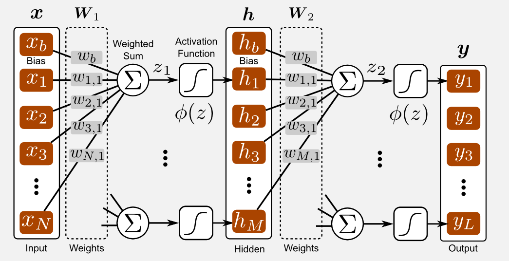
The MLP in its classical form, is based on an input layer, an hidden layer and an output layer. The transfer function used between the layers is generally a sigmoid. The error function can be defined as the mean squared error (MSE) between the output and the labels. Each layer of the MLP can be represented as a product between an input vector \(\boldsymbol{x}\) and a weight matrix \(\boldsymbol{W}\). The resulting value is added to a bias and passed to an activation function, generating an output vector \(\boldsymbol{y}\). These operations are equivalent to the weighted sum of the input values used for the linear approximators. Similarly to the Perceptron we can represent an MLP as a directed graph. In the following image (that I suggest you to look very carefully) you can see how an MLP is assembled. The main difference with respect to the Perceptron is the hidden layer \(h\) that is obtained through the product of the input vector \(x\) and the weight matrix \(W_{1}\). After the weighted sum the array \(z\) is passed through a sigmoid activation function. You should notice how the bias term is embedded in both the input and hidden vectors. The same process is repeated another time. The output of the hidden layer is multiplied with the weight matrix \(W_{2}\), passed through a sigmoid, leading to the final output vector \(y\). In the neural network lingo, the procedure that leads from the input \(x\) to the output \(y\) is called the forward pass.
Why the MLP is not a linear model? This is a crucial point. It can be easily proved that the MLP is a non-linear approximator only if we use a non-linear activation function (e.g. sigmoid, tanh, ReLU, etc). If we replace the sigmoid with a linear activation then our MLP collapses into a Perceptron. Another interesting fact about the MLP is that given a sufficient amount of hidden neurons it can approximate any continuous function. This is known as the universal approximation theorem and it was proved by George Cybenko in 1989.
Backpropagation (overview)
The main innovation behind the MLP is the update rule which is based on backpropagation. The idea of backpropagation was not completely new at that time, but finding out that it was possible to apply it to feedforward networks took a while. As you remember from the previous post each time we want to train a function approximator we need two things:
- An error measure that gives a distance between the output of the estimator and the target.
- An update rule that set the parameters of the estimator in order to reduce the error.
Since neural networks are function approximators they also need these two components. The error measure is still given by the Mean Squared Error (MSE) between the network output and the target value. Since we are using TD(0) with bootstrapping and online updates after each step, this error measure reduces to:
\[\text{MSE}( \boldsymbol{W_{1}, W_{2}} ) = \frac{1}{2} \big[ U^{\sim}(s_{t+1}) - \text{MLP}(s_{t}) \big]^{2}\]using bootstrapping the target utility function \(U^{\sim}\) is estimated by the MLP itself at \(t+1\) and weighted by the discount factor \(\gamma\) plus the reward, leading to the following expression:
\[\text{MSE}( \boldsymbol{W_{1}, W_{2}} ) = \frac{1}{2} \big[ r_{t+1} + \gamma \text{MLP}(s_{t+1}) - \text{MLP}(s_{t}) \big]^{2}\]The update rule is still an application of the gradient descent procedure, that in the neural network context is called backpropagation. It is necessary to remember that bootstrapping ignores the effect on the target, taking into account only the partial derivatives of the estimation at \(s_{t}\) with respect to the weights \(W_{1}\) and \(W_{2}\) (semi-gradient method). If you do not want to get into the mathematical details of backpropagation this is enough, and you can skip the next section.
Backpropagation (some math)
It is possible to think about backpropagation as an iterative application of the chain rule on the different layers of the network. If you want to understand the math behind backpropagation you should refresh your calculus. Here I can only give you a quick recap based on the material I used in introductory courses for undergraduates. First of all, it is mandatory to know what is a derivative and how to calculate the derivative of the most important functions (e.g. sin, cos, exponential, polynomials). The chain rule is a simple iterative process that allows computing the derivative of a composition of functions. The iterative process consists in moving through the composition and estimating the derivatives of all the functions encountered along the way. Here I will show you an example of chain rule applied to an equation having a single variable \(x\):
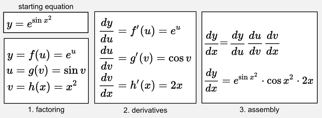
As you can see the idea is to (1) factor the starting equation in different parts, then (2) estimate the derivative of each part, and finally (3) multiply each part. Intuitively you can see backpropagation as the process of opening a set of black Chinese boxes until a red box appear. In our example the red box is the variable \(x\) and the black boxes to open are the various equations we have to derive in order to reach it.
How does the chain rule fit into neural networks? This is something many people struggle with. Consider the neural network as a magic box where you can push an array, and get back another array. Push an input, get an output. Input and output can have different size, in our Perceptron for instance, the input array consisted of 400 values and the output was a single value. This is technically a scalar field. In our examples of MLP we will feed an array representing the world state, and we will get an output representing the utility of that state (as a single value), or the utility of each possible action (as an array). Now, a neural network is not a magic box. The output \(y\) is obtained through a series of operation. If you carefully look at the MLP scheme of the previous section you can go back from \(y\) to \(h\) and from \(h\) to \(x\). In the end, \(y\) is obtained from applying a sigmoid to the weighted sum of \(h\) and a set of weights. Whereas \(h\) is obtained in a similar way using the weighted sum of \(x\) and the first matrix of weights. This long chain of operation is a composition of multiple functions, and by definition we can apply the chain rule to it.
Where are the variables in a neural network? In a neural network we do not have only a single variable to estimate, the variables (or unknowns) of our network are the weights that connect the units. Our goal is to find the set of weights that better represent the real utility function. Differently from a single variable equation (like the one used in the chain rule example above) a neural network is a multivariable equation. For instance, you can think of the Rosenblatt’s Perceptron as a multivariable equation having 400 unknowns. In a multivariable equation we do not think in terms of derivative but in terms of gradient. I already wrote about gradient in the previous post. Dealing with a multivariable equation is not something that should scare you, since our chain rule still works. However, we now need to use partial derivatives instead of standard derivatives. Given the error function \(E\) we have to look for the set of variables \(\boldsymbol{W}_{1}\) and \(\boldsymbol{W}_{2}\), meaning that we keep differentiating (opening the Chinese boxes) until we do not find them. In the image below you can find a mathematical description of this process for a MLP having a vector \(x\) as input, a vector \(y\) as output, two set of weights \(W_{1}\) (between input and hidden layers) and \(W_{2}\) (between hidden and output layers). the weighted sum of these components generate two arrays \(z_{1}\) and \(z_{2}\) and passed through two activation functions \(h = \phi(z_{1})\) and \(y = \phi(z_{2})\). Remember that the last link of the chain is the error function \(E\), and for this reason \(E\) is the starting point for the chain rule.
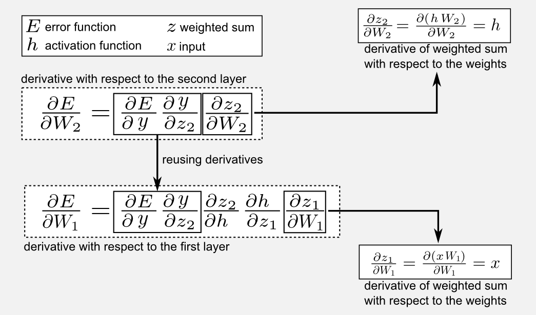
As you can notice the use of backpropagation is very efficient because it allows us to reuse part of the partial derivatives computed in later layers in order to estimate the derivatives of previous layers. Moreover all those operations can be formalised in matrix-vector form and can be easily parallelised on a GPU.
What does backpropagation return? The backpropagation finds the gradient vectors of the unknowns. In our MLP the backpropagation finds two vectors, one for the weights \(W_{1}\) and the other for the weights \(W_{2}\). Great, but how should we use those vectors? If you remember from the last post the gradient vector is the vector pointing up-hill on the error surface, meaning that it shows us where we should move in order to reach the top of the function. However here we are interested in going down-hill because we want to minimize an error (in the end we are doing gradient descent). This change in direction can be easily achieved changing the sign in front of the gradient.
Now, knowing the direction in which to move the weights is not enough, we need to know how much we have to move in that direction. You must recall that the steepness of the function at a specific point is given by the magnitude of the gradient vector. From your linear algebra class you should know that multiplying a vector by a scalar changes the magnitude of the vector. This scalar step is called learning rate. Finding an optimal learning rate is not easy. Researcher generally uses a linear decay to decrease the value of the learning rate. Today there are techniques (e.g. Adagrad, Adam, RMSProp, etc) that can dynamically adjust the learning rate based on the slope of the error surface. Give a look to this well written blog post if you want to know more about adaptive gradient methods.
From bla-bla-bla to Python
Implementing a multilayer perceptron in Python is very easy if we think in terms of matrices and vectors. The input is a vector \(x\), the weights of the first layer are a matrix \(W1\), the weights of the second layer a matrix \(W2\). The forward pass can be represented as matrix-vector product between \(x\) and \(W1\). the product produces an activation in the hidden layer called \(h\), and this vector is then used to produce the output \(y\) through the product with \(W2\) the weight matrix in the second layer. I will embedd everything in a class called MLP, that we are going to use later. Here I describe the methods of the class, you can find the complete code in the GitHub repository and the MLP class in the script called mlp.py. Let’s start with the __init__() method:
def __init__(self, tot_inputs, tot_hidden, tot_outputs):
    '''Init an MLP object

    Defines the matrices associated with the MLP.
    @param: tot_inputs
    @param: tot_hidden
    @param: tot_outputs
    '''
    import numpy as np
    if(activation!="sigmoid" and  activation!="tanh"):
        raise ValueError("[ERROR] The activation function "
                         + str(activation) + " does not exist!")
    else:
        self.activation = activation
    self.tot_inputs = tot_inputs
    self.W1 = np.random.normal(0.0, 0.1, (tot_inputs+1, tot_hidden))
    self.W2 = np.random.normal(0.0, 0.1, (tot_hidden+1, tot_outputs))
    self.tot_outputs = tot_outputs
You should notice how I added the bias as an additional row in the weight matrices when I wrote tot_inputs+1 and tot_hidden+1. As explained in this post and the previous, the bias is an additional unit in both the input vector \(x\) and the hidden activation \(h\). The weights of the matrix are randomly initialised from a Gaussian distribution with mean 0.0 and standard deviation 0.1. Great, we can now give a look to the other methods of the class: activation functions and forward pass.
def _sigmoid(self, z):
    return 1.0 / (1.0 + np.exp(-z))

def _tanh(self, z):
    return np.tanh(z)

def forward(self, x):
    '''Forward pass in the neural network

    Forward pass via dot product
    @param: x the input vector (must have shape==tot_inputs)
    @return: the output of the network
    '''
    self.x = np.hstack([x, np.array([1.0])]) #add the bias unit
    self.z1 = np.dot(self.x, self.W1)
    if(self.activation=="sigmoid"):
        self.h = self._sigmoid(self.z1)
    elif(self.activation=="tanh"):
        self.h = self._tanh(self.z1)
    self.h = np.hstack([self.h, np.array([1.0])]) #add the bias unit
    self.z2 = np.dot(self.h, self.W2) #shape [tot_outputs]
    if(self.activation=="sigmoid"):
        self.y = self._sigmoid(self.z2)
    elif(self.activation=="tanh"):
        self.y = self._tanh(self.z2)
    return self.y
There are a few things to notice. I added the bias unit using the Numpy method hstack(). This has been done for both the input and the hidden activation. I added two activation functions: sigmoid and hyperbolic tangent (tanh). The difference between the two is in the output, the sigmoid has an output in the range \([0, 1]\) whereas the tanh has an output in the range \([-1, 1]\). You can expand the number of functions including additional methods. Now the backward pass:
def _sigmoid_derivative(self, z):
    return self._sigmoid(z) * (1.0 - self._sigmoid(z))

def _tanh_derivative(self, z):
    return 1 - np.square(np.tanh(z))

def backward(self, y, target):
    '''Backward pass in the network

    @param y: the output of the network in the forward pass
    @param target: the value of taget vector (same shape of output)
    '''
    if(y.shape!=target.shape):
        raise ValueError("[ERROR] The size of target is wrong!")
    #gathering all the partial derivatives
    dE_dy = -(target - y)
    if(self.activation=="sigmoid"):
        dy_dz2 = self._sigmoid_derivative(self.z2)
    elif(self.activation=="tanh"):
        dy_dz2 = self._tanh_derivative(self.z2)
    dz2_dW2 = self.h
    dz2_dh = self.W2
    if(self.activation=="sigmoid"):
        dh_dz1 = self._sigmoid_derivative(self.z1)
    elif(self.activation=="tanh"):
        dh_dz1 = self._tanh_derivative(self.z1)
    dz1_dW1 = self.x
    #gathering the gradient of W2
    dE_dW2 = np.dot(np.expand_dims(dE_dy * dy_dz2, axis=1),
                    np.expand_dims(dz2_dW2, axis=0)).T
    #gathering the gradient of W1
    dE_dW1 = (dE_dy * dy_dz2)
    dE_dW1 = np.dot(dE_dW1, dz2_dh.T)[0:-1] * dh_dz1
    dE_dW1 = np.dot(np.expand_dims(dE_dW1,axis=1),
                    np.expand_dims(dz1_dW1,axis=0)).T
    return dE_dW1, dE_dW2
The backward method returns the gradient vectors necessary to update the network. Here I used a coherent convention for the partial derivatives that is in line with the names used in previous sections of the post, in this way it is possible to match the code and the math. Finally, we have to use both forward and backward pass for the training procedure:
def train(self, x, target, learning_rate=0.1):
    '''train the network

    @param x: the input vector
    @param target: the target value vector
    @param learning_rate: the learning rate (default 0.01)
    @return: the error RMSE
    '''
    y = self.forward(x)
    dE_dW1, dE_dW2 = self.backward(y, target)
    #update the weights
    self.W2 = self.W2 - (learning_rate * dE_dW2)
    self.W1 = self.W1 - (learning_rate * dE_dW1)
    #estimate the error
    error = 0.5 * (target - y)**2
    return error
This is the essential code for a basic MLP, you can extend it adding more layers and error/activation functions. It is important to notice that the current version of the code does not include mini-batch training. For the purpose of this post a single input-target pair is enough, but generally stochastic gradient descent needs a mini-batch of multiple samples which is representative of the function we want to approximate. Expanding the class methods it would be possible to include mini-batch training. There are two ways I can think of. (i) One way is to pass a list of input-target pairs to the method train() and to iterate on those pairs accumulating gradients through the backward() method, then apply the average gradients on the two matrices W1 and W2. (ii) A second alternative is to exploit the Numpy capabilities and implement a tensor-based version of the methods forward() and backward(). This means we have to add another dimension representing the mini-batch, similarly to frameworks such as Tensorflow and pyTorch.
Let’s consider it as another homework…
Application: Multi Layer XOR
In the last post we saw how the XOR problem was impossible to solve using a linear function approximator. Now we have a new tool, multi-layer neural networks, that are powerful non-linear approximators able to solve the XOR problem. Here, I will use an architecture similar to the one used by Rumelhart and al. to solve the XOR problem.
Before moving forward let’s see a quick recap. A neural network is a non-linear function approximator. Similarly to the linear approximator introduced in the previous post, training a neural network requires two components, and error measure and an update rule:
Error Measure: a common error measure is given by the Mean Squared Error (MSE) between two quantities.
Update rule (backprop): the update rule for neural networks is based on gradient descent and it gathers the gradient vectors through a process called backpropagation. Backpropagation is an application of the chain rule.
We can use a neural network to approximate an utility function in a reinforcement learning problem. Here we have our usual cleaning robot, that is moving in a gridworld with 25 states. Using a standard table we would need 25 cells to store in memory all the utilities. Moreover, we should visit all the 25 states to gather those values. Here we use an MLP to solve both those issues. An MLP with 2 inputs, 2 hidden, and 1 output, has a total of 4+2=6 connections to store in memory (9+3=12 when the bias is used). We saved memory space! Moreover, using an MLP we do not need to visit all the 25 cells of the grid-world, because we can approximate the function generalizing to unseen states.

For this example I used a network with 2 inputs, 2 hidden units, and 1 output. I used tanh activation functions for the two layers, this is important because our utility function is in the range [-1, +1] and a sigmoid could not approximate it. For the reinforcement learning part I used the same code of the previous post and similar (quick and dirty) plotting code in matplotlib to show the result. You can find the full code in the GitHub repository under the name xor_mlp_td.py. We can use the MLP class to define a new network called my_mlp and then train the network to approximate the utility function.
def main():
  env = init_env()
  my_mlp = MLP(tot_inputs=2, tot_hidden=2, tot_outputs=1, activation="tanh")
  learning_rate = 0.1
  gamma = 0.9
  tot_epoch = 10001
  #One epoch is one episode
  for epoch in range(tot_epoch):
      observation = env.reset(exploring_starts=True)
      #The episode starts here
      for step in range(1000):
          action = np.random.randint(0,4)
          new_observation, reward, done = env.step(action)
          #call the update method and then the my_mlp.train() method
          #the update() returns the new MLP and the RMSE error
          my_mlp, error = update(my_mlp, new_observation, reward,
                                 learning_rate, gamma, done)
          observation = new_observation
          if done: break
The code above is similar to the one used for the linear and hyperbolic approximators. I run the training for 10000 steps with a learning rate of 0.1 and a gamma of 0.9. Feeding the neural network with a grid of x-y tuples we can obtain the approximated utility function as output and plot it, here we go:
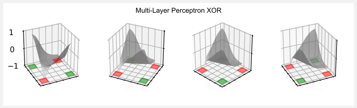
Such a simple neural network can generate a pretty complex function, that is quite similar to the hyperbolic paraboloid we used in the previous post. The utility matrix obtained in the last epoch is here reported:
Epoch: 10001
[[ 0.81  0.23 -0.36 -0.55 -0.6 ]
 [ 0.49 -0.12 -0.42 -0.49 -0.5 ]
 [ 0.01 -0.18 -0.21 -0.16 -0.1 ]
 [-0.44 -0.02  0.28  0.45  0.54]
 [-0.87 -0.28  0.43  0.7   0.79]]
In the XOR world, the top-left and bottom-right corners of the matrix have an utility of +1 whereas the top-right and bottom-left corners have an utility of -1. We see that the network captured this trend with values of 0.81, 0.79, -0.87, and -0.6. I got this results without much effort, I think that fine tuning of the hyper-parameters can get us even closer.
Your homework is to change the structure of the network, increasing the size of the hidden layer, and verify how the plot changes. Remember that increasing the number of hidden units increases the degrees of freedom of your approximator. To avoid underfitting and overfitting you must always take into account the bias-variance tradeoff.
Beyond the Multi Layer Perceptron
Even though using an MLP can give a large advantage in many problems, there are still some major limitations we did not discuss. Here I list three of them:
-
Size of the model. The fully-connected layer of an MLP has a number of parameters that grows rapidly with the number of units. It would be better to have shared weights.
-
Update rule. Training a neural network with stochastic gradient descent requires samples that are independent and identically distributed (i.i.d.). However, the samples gathered from our grid-world are strongly related.
-
Instability. Training a neural network can be very unstable in some reinforcement learning algorithms (see for instance Q-learning and its bootstrap mechanism).
It took several years to find a solution to all these problems, however a stable algorithm has been recently developed. I am talking about deep reinforcement learning, the topic of the next post.
Bonus: policy gradient methods
As bonus material I would like to provide a quick overview on another reinforcement learning approach that widely uses neural netwokrs. Until now we approximated the utility (or state-action) function. However there is another way to go: the approximation of the policy. At the end of the fourth post I explained what is the difference between an actor-only and a critic-only algorithm. The policy gradient is an actor-only method that aims to approximate the policy. Before moving forward it may be useful to recap what is the difference between utility, state-action, and policy functions:
- Utility (or value) function: \(y = U(s)\) receives as input a state vector \(s\) and return the utility \(y\) of that state.
- State-action function: \(y = Q(s, a)\) receives as input a state \(s\) and an action \(a\), and returns the utility \(y\) of that state-action pair.
- Policy function: \(a = \pi(s)\) receives as input a state \(s\) and returns the action to perform in that state.
In policy gradient methods we use a neural network to approximate the policy function \(\pi(s)\). As the name suggest we are using the gradient. At this point of the series you should know what is the gradient vector and how we are using it in gradient descent methods. Here, we want to estimate the gradient of our neural network, but we do not want to minimise an error anymore. Instead we want to maximise the expected return (long-term cumulative reward). As I told you before the gradient indicates the direction we should move the weights in order to maximise a function, and this is exactly what we want to achieve in policy gradient methods.
Advantages: the main advantage of policy gradient methods is that in some context it is much easier to estimate the policy function instead of the utility function. We know that the estimation of the utility function can be difficult due to the credit assignment problem. In policy gradients method we bypass this issue and we obtain a better convergence and an increased stability. Another advantage is that using policy gradient we can approximate a continuous action space. This overcomes an important limitation of Q-Learning where the \(max\) operator only allows us to approximate discrete action spaces (see third post for more details).
Disadvantages: the main disadvantage of policy gradient methods is that they are generally slower and that they often converge to local optimum. Another problem is variance. Evaluating the policy with an high number of trajectories leads to an high variance in the approximation of the function.
One of the most widely used policy gradient methods is called REINFORCE, and it is based on a Monte Carlo approach. The REINFORCE algorithm finds an unbiased estimate of the gradient without using any utility function. I hope to have time to describe REINFORCE in a future post, for the moment you can give a look to the scholarpedia page if you want to know more.
Conclusions
In this post we saw how feed forward neural networks work and how they can be used to approximate an utility function. Recent advancements have moved beyond MLP with the use of Convolutional Neural Networks and stable training techniques. The most impressive results have been obtained in challenging problems such as ATARI games and the ancient game of GO. In the next post we will see how Deep Reinforcement Learning can be used to tackle some of those problems.
Index
- [First Post] Markov Decision Process, Bellman Equation, Value iteration and Policy Iteration algorithms.
- [Second Post] Monte Carlo Intuition, Monte Carlo methods, Prediction and Control, Generalised Policy Iteration, Q-function.
- [Third Post] Temporal Differencing intuition, Animal Learning, TD(0), TD(λ) and Eligibility Traces, SARSA, Q-learning.
- [Fourth Post] Neurobiology behind Actor-Critic methods, computational Actor-Critic methods, Actor-only and Critic-only methods.
- [Fifth Post] Evolutionary Algorithms introduction, Genetic Algorithm in Reinforcement Learning, Genetic Algorithms for policy selection.
- [Sixt Post] Reinforcement learning applications, Multi-Armed Bandit, Mountain Car, Inverted Pendulum, Drone landing, Hard problems.
- [Seventh Post] Function approximation, Intuition, Linear approximator, Applications, High-order approximators.
- [Eighth Post] Non-linear function approximation, Perceptron, Multi Layer Perceptron, Applications, Policy Gradient.
Resources
-
The complete code for the Reinforcement Learning Function Approximation is available on the dissecting-reinforcement-learning official repository on GitHub.
-
Reinforcement learning: An introduction (Chapter 8 ‘Generalization and Function Approximation’) Sutton, R. S., & Barto, A. G. (1998). Cambridge: MIT press. [html]
-
Policy gradient methods on Scholarpedia by Prof. Jan Peters [wiki]
-
Tensorflow playground, try different MLP architectures and datasets on the browser [web]
References
Goodfellow, I., Bengio, Y., Courville, A., & Bengio, Y. (2016). Deep learning. Cambridge: MIT press.
Hebb, D. O. (2005). The first stage of perception: growth of the assembly. In The Organization of Behavior (pp. 102-120). Psychology Press.
Minsky, M., & Papert, S. A. (2017). Perceptrons: An introduction to computational geometry. MIT press.
Rumelhart, D. E., Hinton, G. E., & Williams, R. J. (1986). Learning representations by back-propagating errors. nature, 323(6088), 533.
Sutton, R. S., McAllester, D. A., Singh, S. P., & Mansour, Y. (2000). Policy gradient methods for reinforcement learning with function approximation. In Advances in neural information processing systems (pp. 1057-1063).