Dissecting Reinforcement Learning-Part.7
So far we have represented the utility function by a lookup table (or matrix if you prefer). This approach has a problem. When the underlying Markov decision process is large there are too many states and actions to store in memory. Moreover in this case it is extremely difficult to visit all the possible states, meaning that we cannot estimate the utility values for those states. The key issue is generalization: how to produce a good approximation of a large state space experiencing only a small subset. In this post I will show you how to use a linear combination of features in order to approximate the utility function. This new technique will allow us to master new and old problems more efficiently. For example, in this post you will learn how to implement a linear version of the TD(0) algorithm and how to use it to find the utilities of multiple gridworlds.
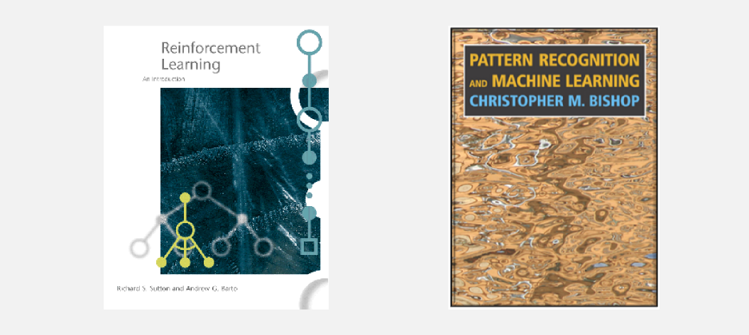
The reference for this post is chapter 8 for the Sutton and Barto’s book called “Generalization and Function Approximation”. Moreover a good resource is the video-lesson 6 of David Silver’s course. A wider introduction to function approximation is given by any good machine learning textbook, I suggest Pattern Recognition and Machine Learning by Christopher Bishop. I want to start this post with a brief excursion in the neuroscience world. Let’s see how a function approximator relates to biological brains.
Approximators (and grandmothers)
You couldn’t read this post without using a powerful approximator: your brain. The first primordial brains, a bunch of nerve cells, gave a great advantage allowing elementary creatures to better perceive and react, considerably extending their lifespan. Evolution shaped brains for thousands of years optimising size, modularity, and connectivity. Having a brain seems a big deal. Why? What’s the purpose of having a brain? We can consider the world as a huge and chaotic state-space, where the correct evaluation of a specific stimulus makes the difference between life and death. The brain stores information about the environment and allows an effective interaction with it. Let suppose that our brain is a massive lookup table, which can store in a single neuron (or cell) a single state. This is known as local representation. This theory is often called the grandmother cell. A grandmother cell is a hypothetical neuron that responds only to a specific and meaningful stimulus, such as the image of one’s grandmother. The term is due to the cognitive scientist Jerry Lettvin who used it to illustrate the inconsistency of the concept during a lecture at MIT. To describe the grandmother cell theory I will use the following example. Let’s suppose we bring a subject in an isolated room. The activity of a group of neurons in the subject brain is constantly monitored. In front of the subject there is a screen. Showing to the subject the picture of his grandmother we notice that a specific neuron fires. Showing the grandmother in different contexts (e.g. in a group picture) activates again the neuron. However showing on screen a neutral stimulus does not activate the neuron.

During the 1970s the grandmother cell moved into neuroscience journals and a proper scientific discussion started. In the same period Gross et al. (1972) observed neurons in the inferior temporal cortex of the monkey that fired selectively to hands and faces. The grandmother cell theory started to be seriously taken into account. The theory was appealing because simple to grasp and pretty intuitive. However a theoretical analysis of the grandmother cell confirmed many underlying weaknesses. For instance, in this framework the loss of a cell means the loss of a specific chunk of information. Basic neurobiological observations strongly suggest the opposite. It is possible to hypothesise multiple grandmother cells, which codify the same information in a distributed way. Redundancy prevents loss. This explanation complicate even more the situation, because storing a single state requires multiple entries in the lookup table. To store \(N\) states without the risk of information loss, at least \(2 \times N\) cells are required. The paradox of the grandmother cell is that trying to simplify the brain functioning, it finishes to complicate it.
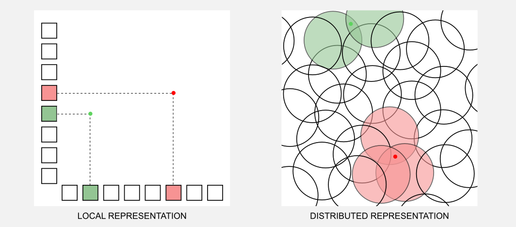
There is an alternative to the grandmother cell hypothesis? We can suppose that information is stored in a distributed way, and that each single concept is represented through a pattern of activity. This theory was strongly sustained by researchers such as Geoffrey Hinton (one of the “godfather” of deep learning), and James McClelland. The distributed representation theory gives a big advantage. Having \(N\) cells it is possible to represent more than \(N\) states, whereas this is not true for a local representation. Moreover a distributed representation is robust against loss and it guaranties an implicit redundancy. Even though each active unit is less specific in its meaning, the combination of active units is far more specific. To understand the difference between the two representations think about a computer keyboard. In the local representation each single key can codify only a single character. In the distributed representation we can use a combination of keys (e.g. Shift and Ctrl) to associate multiple characters to the same key. In the image below (inspired by Hinton, 1984) is represented how two stimuli (red and green dots) are codified in a local and distributed scheme. The local scheme is represented as a two dimensional grid, where it is always necessary to have two active units to codify a stimulus. We can think the distributed representation as an overlapping between radial units. The two stimuli are codified through an high level pattern given by the units enclosed in a specific activation radius.
How is it possible to explain the monkey selective-neurons described by Gross et al. (1972) using a distributed representation? A selective-neuron can be the visible part of an underlying network which encapsulate the information. Further research showed that those selective neurons had a large variation in their responsiveness and that it was connected to different aspects of faces. This observation suggested that those neurons embedded a distributed representation of faces.
If you think that the grandmother cell theory is something born and dead in the Seventies you are wrong. In recent years the local representation theory received support from biological observations (see Bowers 2009), however these results have been strongly criticised by Plaut and McClelland (2009). For a very recent survey I suggest you this article. From a machine learning perspective we know that the distributed representation works. The success of deep learning is based on neural networks, which are powerful function approximators. Moreover different methods, such as dropout, are tightly related to the distributed representation theory. Now it’s time to go back to reinforcement learning, and see how a distributed representation can solve the problems due to local representation.
Function approximation intuition
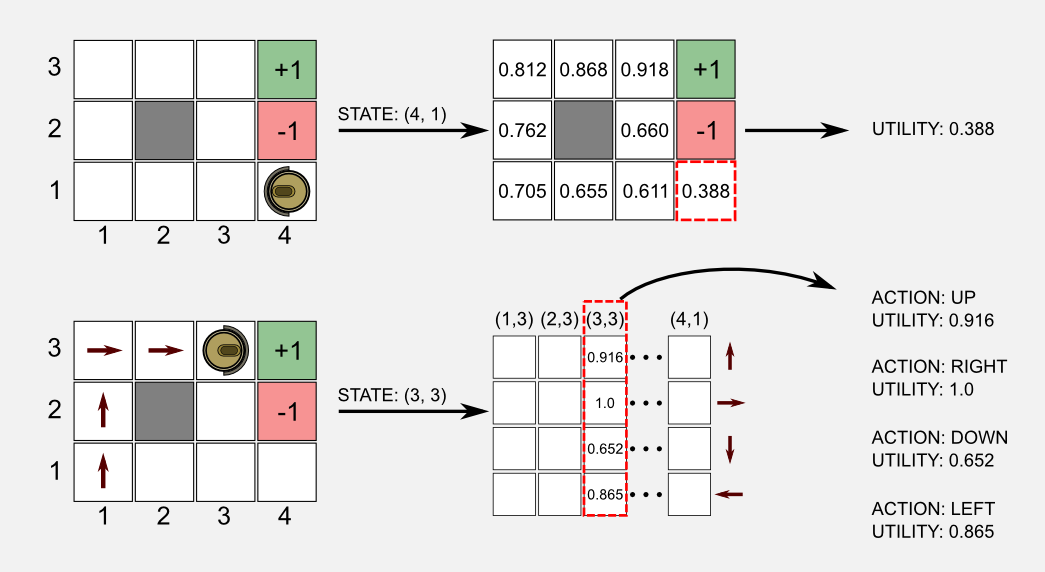
Here I will use again the robot cleaning example described in previous posts. The robot moves in a two-dimensional world we called gridworld. It has only 4 possible actions available (forward, backward, left, right) and its goal is to reach a charger (green cell) and avoid to fall on stairs (red cell). I define with \(U(s)\) our usual utility function, and with \(Q(s,a)\) the state-action function. The grid-world is a discrete rectangular state space, having \(c\) columns and \(r\) rows. Using a tabular approach we can represent \(U(s)\) using a table containing \(r \times c = N\) elements, where \(N\) represent the total number of states. To represent \(Q(s,a)\) we need a table of size \(N \times M\), where \(M\) is the total number of actions. In the previous posts I always represented the lookup tables using matrices. As utility function I used a matrix having the same size of the world, whereas for the state-action function I used a matrix having \(N\) columns (states) and \(M\) rows (actions). In the first case, to get the utility we have to access the location of the matrix corresponding to the particular state where we are. In the second case, we use the state as index to access the column in the state-action matrix and from that column we return the utilities of all the available actions.
How can we fit the function approximation mechanism inside this scheme? Let’s start with some definitions. Defining as \(S= \{ s_{1}, s_{2}, ... , s_{N} \}\) the set of possible states, and as \(A= \{ a_{1}, a_{2}, ... , a_{M} \}\) the set of possible actions, we define a utility function approximator \(\hat{U}(S,\boldsymbol{w})\) having parameters stored in a vector \(\boldsymbol{w}\). Here I use the hat on top of \(\hat{U}\) to differentiate this function from the tabular version \(U\).
Before explaining how to create a function approximator it is helpful to visualise it as a black box. The method described below can be used on different approximators and for this reason we can easily apply it to the box content. The black box takes as input the current state and returns the utility of the state or the state-action utilities. That’s it. The main advantage is that we can approximate (with an arbitrary small error) the utilities using less parameters respect to the tabular approach. We can say that the number of elements stored in the vector \(\boldsymbol{w}\) is smaller than \(N\) the number of values in the tabular counterpart.
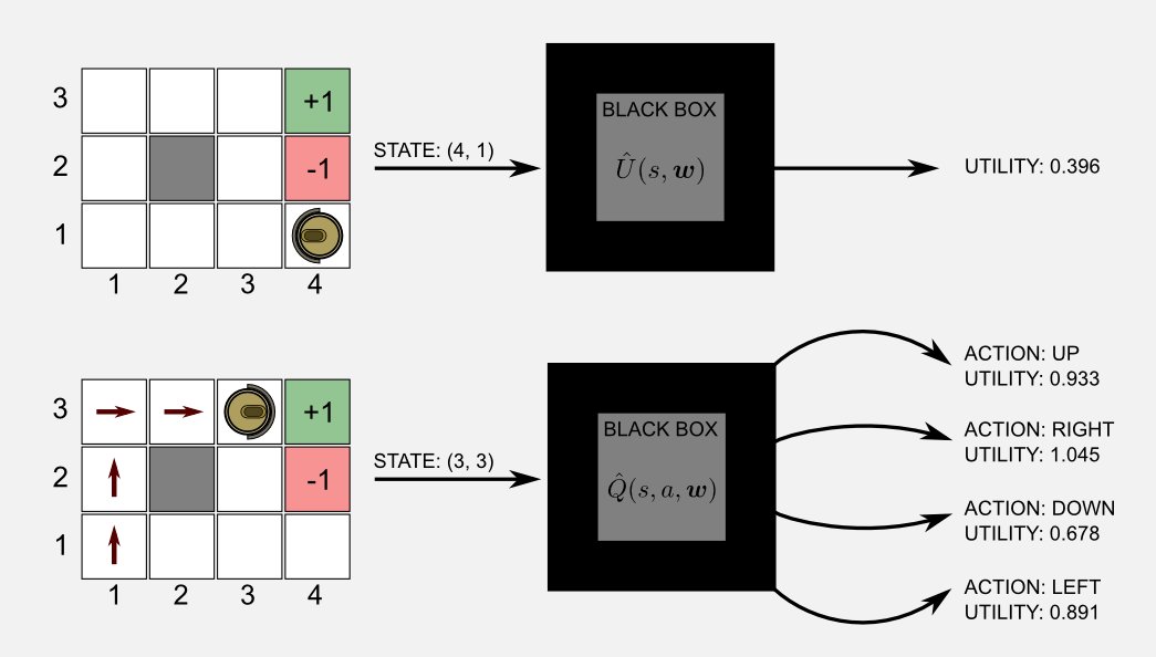
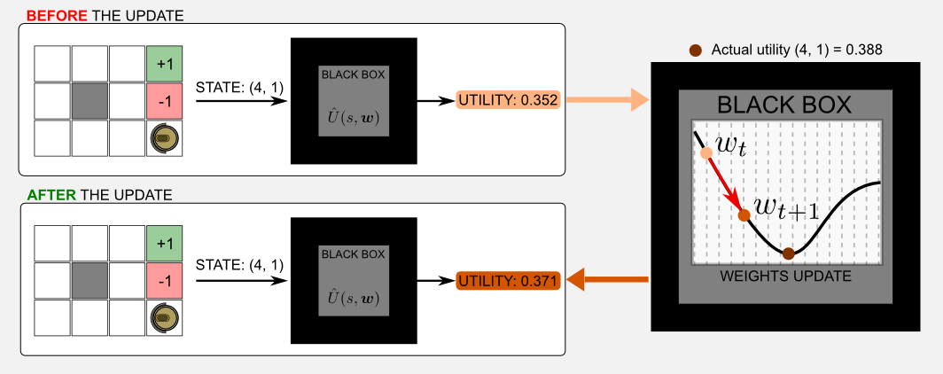
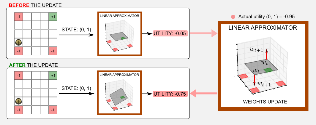
I guess there is a question that came to your head: what there is inside the black box? This is a legitimate question and now I will try to give you the intuition. In the case of a blackbox that is approximating an utility function, the content of the box is \(\hat{U}(s, \boldsymbol{w})\). You can imagine the utility function as a music mixer and the vector of weights \(\boldsymbol{w}\) as the mixer sliders. We want to adjust the sliders in order to obtain a sound which is similar to a predefined tone. How to do it? Well we can move one of the slider and compare the output with the reference tone. If the output is more similar to the reference we know that we moved the right slider. Repeating this process many times we eventually obtain a tone which is very similar to the reference sound. Using a more formal view we can say that the vector \(\boldsymbol{w}\) is adjusted at every iteration, moving the values of a quantity \(\Delta\), in order to reach an objective which is minimising a function of cost. The cost is given by an error measure that we can obtain comparing the output of the function with a target. For instance, we know from previous posts that the actual utility value of state (4,1) in our gridworld is 0.388. Let’s say that at time \(t\) the output of the box is 0.352. After the update step the output will be 0.371, we moved closer to the target value.
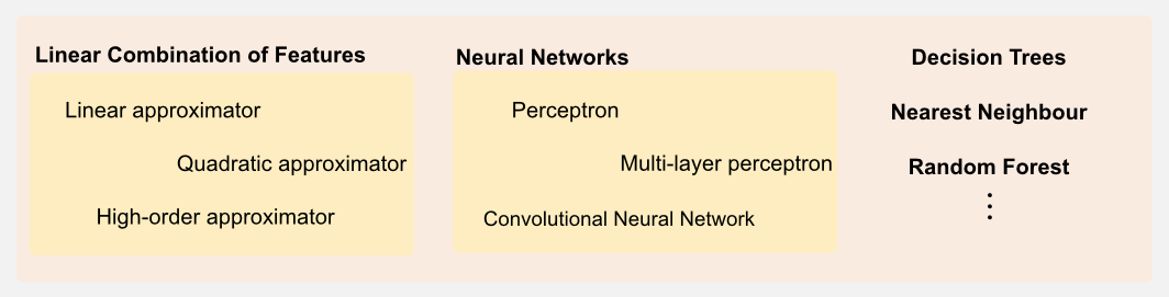
Function approximation is an instance of supervised learning. In principle all the supervised learning techniques could be used in function approximation. The vector \(\boldsymbol{w}\) may be the set of connection weights of a neural network or the split points and leaf values of a decision tree. However here I will consider only differentiable function approximators such as linear combination of features and neural networks, which represents the most promising techniques nowadays. In this post I will focus on linear combination of features.
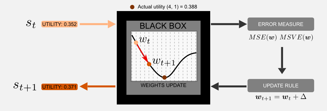
Before describing the simplest case the linear approximator, I would like to introduce the general methodology used to adjust the vector of weights. The goal in function approximation is to move as close as possible to the real utility function adjusting the internal parameters stored in \(\boldsymbol{w}\). To achieve this goal we need two things, first an error measure that can give us a feedback on how close we are to the target, second an update rule for adjusting the weights. In the next section I will describe these two components.
Method
To improve the performance of our function approximator we need an error measure and an update rule. These two components work tightly in the learning cycle of every supervised learning technique. Their use in reinforcement learning is not much different from how they are used in a classification task. In order to understand this section you need to refresh some concepts of multivariable calculus such as the partial derivative and gradient.
Error Measure: a common error measure is given by the Mean Squared Error (MSE) between two quantities. For instance, if we have the optimal utility function \(U^{*}(S)\) and an approximator function \(\hat{U}(s, \boldsymbol{w})\), then the MSE is defined as follows:
\[\text{MSE}( \boldsymbol{w} ) = \frac{1}{N} \sum_{s \in S} \big[ U^{*}(s) - \hat{U}(s, \boldsymbol{w}) \big]^{2}\]that’s it, the MSE is given by the expectation \(\mathop{\mathbb{E}}[ (U^{*}(s) - \hat{U}(s, \boldsymbol{w}) \big)^{2} ]\) that quantifies the difference between the target and the approximator output. When the training is working correctly the MSE will decrease meaning that we are getting closer to the optimal utility function. The MSE is a common loss function used in supervised learning. However, in reinforcement learning it is often used a reinterpretation of the MSE called Mean Squared Value Error (MSVE). The MSVE introduce a distribution \(\mu(s) \geq 0\) that specifies how much we care about each state \(s\). As I told you the function approximator is based on a set of weights \(\boldsymbol{w}\) that contains less elements than the total number of states. For this reason adjusting a subset of the weights means improving the utility prediction of some states but loosing precision in others. We have limited resources and we have to manage them carefully. The function \(\mu(s)\) gives us an explicit solution and using it we can rewrite the previous equation as follows:
\[\text{MSVE}( \boldsymbol{w} ) = \frac{1}{N} \sum_{s \in S} \mu(s) \big[ U^{*}(s) - \hat{U}(s, \boldsymbol{w}) \big]^{2}\]Update rule: the update rule for differentiable approximator is gradient descent. The gradient is a generalisation of the concept of derivative applied to scalar-valued functions of multiple variables. You can imagine the gradient as the vector that points in the direction of the greatest rate of increase. Intuitively, if you want to reach the top of a mountain the gradient is a signpost that in each moment show you in which direction you should walk. The gradient is generally represented with the operator \(\nabla\) also known as nabla. The goal in gradient descent is to minimise the error measure. We can achieve this goal moving in the direction of the negative gradient vector, meaning that we are not moving anymore to the top of the mountain but downslope. At each step we adjust the parameter vector \(\boldsymbol{w}\) moving a step closer to the valley. First of all, we have to estimate the gradient vector for \(\text{MSE}( \boldsymbol{w} )\) or \(\text{MSVE}( \boldsymbol{w} )\). Those error functions are based on \(\boldsymbol{w}\). In order to get the gradient vector we have to calculate the partial derivative of each weight with respect to all the other weights. Secondly, once we have the gradient vector we have to adjust the value of all the weights in accordance with the negative direction of the gradient. In mathematical terms, we can update the vector \(\boldsymbol{w}\) at \(t+1\) as follows:
\[\begin{eqnarray} \boldsymbol{w}_{t+1} &=& \boldsymbol{w}_{t} - \frac{1}{2} \alpha \nabla_{\boldsymbol{w}} \text{MSE}(\boldsymbol{w}_{t}) \\ &=& \boldsymbol{w}_{t} - \frac{1}{2} \alpha \nabla_{\boldsymbol{w}} \big[ U^{*}(s) - \hat{U}(s, \boldsymbol{w}_{t}) \big]^{2}\\ &=& \boldsymbol{w}_{t} + \alpha \big[ U^{*}(s) - \hat{U}(s, \boldsymbol{w}_{t}) \big] \nabla_{\boldsymbol{w}} \hat{U}(s, \boldsymbol{w}_{t}) \\ \end{eqnarray}\]The last step is an application of the chain rule that is necessary because we are dealing with a function composition. We want to find the gradient vector of the error function with respect to the weights, and the weights are part of our function approximator \(\hat{U}(s, \boldsymbol{w}_{t})\). The minus sign in front of the quantity 1/2 is used to change the direction of the gradient vector. Remember that the gradient points to the top of the hill, while we want to go to the bottom (minimizing the error). In conclusion the upate rule is telling us that all we need is the output of the approximator and its gradient. Finding the gradient of a linear approximator is particularly easy, whereas in non-linear approximators (e.g. neural networks) it requires more steps.
At this point you might think we have all we need to start the learning procedure, however there is an important part missing. We supposed it was possible to use the optimal utility function \(U^{*}\) as target in the error estimation step. We do not have the optimal utility function. Think about that, having this function would mean we do not need an approximator at all. Moving in our gridworld we could simply call \(U^{*}(s_{t})\) at each time step \(t\) and get the actual utility value of that state. What we can do to overcome this problem is to build a target function \(U^{\sim}\) which represent an approximated target and plug it in our formula:
\[\boldsymbol{w}_{t+1} = \boldsymbol{w}_{t} + \alpha \big[ U^{\sim}(s) - \hat{U}(s, \boldsymbol{w}) \big] \nabla_{\boldsymbol{w}} \hat{U}(s, \boldsymbol{w})\]How can we estimate the approximated target? We can follow different approaches, for instance using Monte Carlo or TD learning. In the next section I will introduce these methods.
Target estimation
In the previous section we came to the conclusion that we need approximated target functions \(U^{\sim}(s)\) and \(Q^{\sim}(s,a)\) to use in the error evaluation and update rule. The type of target used is at the heart of function approximation in reinforcement learning. There are two main approaches:
Monte Carlo target: an approximated value for the target can be obtained through a direct interaction with the environment. Using a Monte Carlo approach (see the second post) we can generate an episode and update the function \(U^{\sim}(s)\) based on the states encountered along the way. The estimation of the optimal function \(U^{*}(s)\) is unbiased because \(\mathop{\mathbb{E}}[U^{\sim}(s)] = U^{*}(s)\), meaning that the prediction is guaranteed to converge.
Bootstrapping target: the other approach used to build the target is called bootstrapping and I introduced it in the third post. In bootstrapping methods we do not have to complete an episode for getting an estimation of the target, we can directly update the approximator parameters after each visit. The simplest form of bootstrapping target is the one based on TD(0) which is defined as follows:
\[U^{\sim}(s_{t}) = \hat{U}(s_{t+1}, \boldsymbol{w}) \qquad Q^{\sim}(s_{t}, a) = \hat{Q}(s_{t+1}, a, \boldsymbol{w})\]That’s it, the target is obtained through the approximation given by the estimator itself at \(s_{t+1}\).
I already wrote about the differences between the two approaches, however here I would like to discuss it again in the new context of function approximation. In both cases the functions \(U^{\sim}(s)\) and \(Q^{\sim}(s,a)\) are based on the vector of weights \(\boldsymbol{w}\). For this reason the correct notation we are going to use from now on is \(U^{\sim}(s,\boldsymbol{w})\) and \(Q^{\sim}(s,a,\boldsymbol{w})\). We have to be particularly careful when using the bootstrapping methods in gradient-based approximators. Bootstrapping methods are not true instances of gradient descent because they only care about the parameters in \(\hat{U}(s, \boldsymbol{w})\). At training time we adjust \(\boldsymbol{w}\) in the estimator \(\hat{U}(s,\boldsymbol{w})\) based on a measure of error but we are not changing the parameters in the target function \(U^{\sim}(s,\boldsymbol{w})\) based on an error measure. Bootstrapping ignores the effect on the target, taking into account only the gradient of the estimation. For this reason bootstrapping techniques are called semi-gradient methods. Due to this issue semi-gradient methods does not guarantee the convergence. At this point you may think that it is better to use Monte Carlo methods because at least they are guaranteed to converge. Bootstrapping gives two main advantages. First of all they learn online and it is not required to complete the episode in order to update the weights. Secondly they are faster to learn and computationally friendly.
The Generalised Policy Iteration (GPI) (see second post) applies here as well. Let’s suppose we start with a random set of weights. At the very first step the agent follows an epsilon-greedy strategy moving in the state with the highest utility. After the first step it is possible to update the weights using gradient descent. What’s the effect of this adjustment? The effect is to slightly improve the utility function. At the next step the agent follows again a greedy strategy, then the weights are updated through gradient descent, and so on and so forth. As you can see we are applying the GPI scheme again.
Linear approximator
It’s time to put everything together! We have built a method based on an error measure and an update rule and we know how to estimate a target. Now I will show you how to build an approximator, the content of the black box, represented by the function \(\hat{U}(s, \boldsymbol{w})\). I will describe a linear approximator which is the simplest case of linear combinations, whereas in the next section I will describe some high order approximators. Before describing a liner approximator I want to clarify a crucial point in order to avoid a common missunderstanding. The linear approximator is a particular case of the broader class of linear combination of features. A liner combination is based on a polynomial which can be or not a line. Using only a line to discriminate between states can be very limited. Linear combination means that the parameters are linearly combined. We are not saying anything about the input features, which in fact may be represented by and high-order polynomial. Hopefully this distinction will be clear at the end of the post.
In the linear approximator we model the state as a vector \(\boldsymbol{x}\). This vector contains the current state values at time \(t\), these values are called features. There are different notations for the vector \(\boldsymbol{x}\) but the most common are \(\boldsymbol{x}(s_{t})\) and \(\boldsymbol{x}_{t}\), I will use both these notations. The features can be the position of a robot, angular position and speed of an inverted pendulum, configurations of the stones in a Go game, etc. Here I define also \(\boldsymbol{w}\) as the vector of weights (or parameters) of our linear approximator, having the same number of elements of \(\boldsymbol{x}\). Now we have two vectors and we want to use them in a linear function. How to do it? Simple, we have to perform the dot product between \(\boldsymbol{x}\) and \(\boldsymbol{w}\) as follows:
\[\hat{U}(s, \boldsymbol{w}) = \boldsymbol{x}(s)^{T} \boldsymbol{w}\]If you are not used to linear algebra notation don’t get scared. This is equivalent to the following sum:
\[\hat{U}(s, \boldsymbol{w}) = x_{1} w_{1} + x_{2} w_{2} + ... + x_{N} w_{N}\]where \(N\) is the total number of features. Geometrically this solution is represented by a line (in two-dimensional space), a plane (in a three-dimensional space), or an hyper-plane (in hyper-spaces). Now we know the content of the black box, which is given by the product of the vectors \(\boldsymbol{x}\) and \(\boldsymbol{w}\). However in order to apply the method described in the previous section we still need the error measure, the update rule and the target. Using the MSE we can write the error measure as follows:
\[\text{MSE}( \boldsymbol{w} ) = \sum_{s \in S} \big[ U^{\sim}(s, \boldsymbol{w}) - \boldsymbol{x}(s)^{T} \boldsymbol{w} \big]^{2}\]Using the TD(0) definition we can define the target as follows:
\[U^{\sim}(s, \boldsymbol{w}) = \boldsymbol{x}(s_{t+1})^{T} \boldsymbol{w}\]The update rule defined previously can be reused here as well, however we have to introduce the reward \(r_{t+1}\) and the discount factor gamma as required by the reinforcement learning definition:
\[\boldsymbol{w}_{t+1} = \boldsymbol{w}_{t} + \alpha \big[ r_{t+1} + \gamma \boldsymbol{x}(s_{t+1})^{T} \boldsymbol{w} - \boldsymbol{x}(s)^{T} \boldsymbol{w} \big] \nabla_{\boldsymbol{w}} \hat{U}(s, \boldsymbol{w})\]Great, we have almost all we need. I said almost because a last piece is missing. The update rule requires the gradient \(\nabla_{\boldsymbol{w}} \hat{U}(s, \boldsymbol{w})\). How to find it? It turns out that the gradient of the linear approximator simplify to a very nice form. First of all, based on the previous definitions we can rewrite the gradient as follows:
\[\nabla_{\boldsymbol{w}} \hat{U}(s, \boldsymbol{w}) = \nabla_{\boldsymbol{w}} ( x_{1} w_{1} + x_{2} w_{2} + ... + x_{N} w_{N})\]now we have to find the partial derivatives of the function approximator with respect to each single weight \(w_{1}, w_{2}, ..., w_{N}\). For each unknown we have to find the derivative considering the other unknowns as constants. For instance, the partial derivative of the first unknown \(w_{1}\) is simply \(x_{1}\) because all the other values are considered constant values and the derivative of a constant is zero:
\[\frac{\partial \hat{U}}{\partial w_{1}} = x_{1} + 0 + 0 + ... + 0 = x_{1}\]Applying the same process to all the other weights we end up with the following gradient vector:
\[\nabla_{\boldsymbol{w}} \hat{U}(s, \boldsymbol{w}) = \left(\frac{\partial \hat{U}}{\partial w_{1}}, ..., \frac{\partial \hat{U}}{\partial w_{N}} \right) = \left( x_{1},..., x_{N} \right) = \boldsymbol{x}(s)\]That’s it. The gradient is the input vector \(\boldsymbol{x}(s)\). Now we can rewrite the update rule as follows:
\[\boldsymbol{w}_{t+1} = \boldsymbol{w}_{t} + \alpha \big[ r_{t+1} + \boldsymbol{x}(s_{t+1})^{T} \boldsymbol{w} - \boldsymbol{x}(s)^{T} \boldsymbol{w} \big] \boldsymbol{x}(s)\]Great, this is the final form of the update rule for the linear approximator. We have all we need now. Let’s get the party started!
Application: gridworld (and the bias)
Let’s suppose we have a square gridworld where charging stations (green cells) and stairs (red cells) are disposed in multiple locations. The position of the positive and negative cells can vary giving rise to four worlds which I called: OR-world, AND-world, NAND-world, XOR-world. The rule of the worlds are similar to the one defined in the previous posts. The robot has four action available: forward, backward, left, right. When an action is performed, with a probability of 0.2 it can lead to a wrong movement. The reward is positive (+1.0) for green cells, negative (-1.0) for red cells, and null in all the other cases. The index convention for the states is the usual (column, row) where (0,0) represents the cell in the bottom-left corner and (4,4) the cell in the top-right corner.
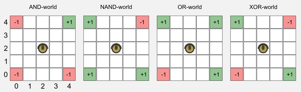
If you are familiar with Boolean algebra you have already noticed that there is a pattern in the worlds which reflects basic Boolean operations. From the geometrical point of view, when we apply a linear approximator to the boolean worlds, we are trying to find a plane in a three-dimensional space which can discriminate between states with high utility (green cells) and states with low utility (red cells).
In the three-dimensional space the x-axis is represented by the columns of the world, whereas the y-axis is represented by the rows. The utility value is given by the z-axis. During the gradient descent we are changing the weights, adjusting the inclination of the plane and the utilities associated to each state. To better understand this point you can plug the equation \(z = x + y\) in Wolfram Alpha and give a look to the resulting plot. Changing the coefficients associated to \(x\) and \(y\) you are changing the weights associated to those features and you are in fact moving the plane. Try again with \(z = \frac{1}{2} x + \frac{1}{4} y\) or click here if you are lazy.
The python implementation is based on a random agent which freely move in the world. Here we are only interested in estimating the state utilities, we do not want to find a policy. The core of the code is the update rule defined in the previous section, summarised in a few lines thanks to Numpy:
def update(w, x, x_t1, reward, alpha, gamma, done):
  '''Return the updated weights vector w_t1

  @param w the weights vector before the update
  @param x the feauture vector obsrved at t
  @param x_t1 the feauture vector observed at t+1
  @param reward the reward observed after the action
  @param alpha the ste size (learning rate)
  @param gamma the discount factor
  @param done boolean True if the state is terminal
  @return w_t1 the weights vector at t+1
  '''
  if done:
    w_t1 = w + alpha * (reward - np.dot(x,w)) * x)
  else:
    w_t1 = w + alpha * ((reward + (gamma*(np.dot(x_t1,w))) - np.dot(x,w)) * x)
  return w_t1
The function numpy.dot() is an implementation of the dot product. The conditional statement is used to discriminate between terminal (done=True) and non-terminal (done=False) states. In case of a terminal state the target is obtained using only the reward. This is obvious, because after a terminal state there is not another state to use for approximating the target.
You can check the complete code on the official GitHub repository of the series, the python script is called boolean_worlds_linear_td.py. In my experiments I set the learning rate \(\alpha = 0.001\) and I linearly decrease it to \(10^{-6}\) for \(3 \times 10^{4}\) iterations. The weights were randomly initialised in the range \([-1,+1]\). Using matplotlib I draw the planes generated for the worlds in a three-dimensional plot:
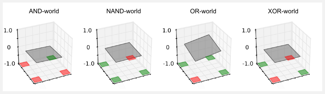
The surface of the plane is the utility value returned by the linear approximator. The utility should be -1 in proximity of a red cell, and +1 in proximity of a green cell. However, examining the plot we can notice that something strange is happening. The planes are flat and the resulting utility is always close to zero in all the worlds but the OR-world. It seems that the approximator is not working at all and that its output is always null. What is going on? Our current definition of approximator does not take into account an important factor, the translation of the plane. Having only two weights we can rotate the surface on the xy-plane but we cannot translate it up and down. This problem becomes clear if you think about the cell (0,0) of the gridworld. The input vector of this cell is \(\boldsymbol{x} = \{ 0, 0 \}\). Given this input, no matter which value we choose for the weights, when we perform the dot product \(\boldsymbol{x}^{T} \boldsymbol{w}\) we are going to end up with an utility of zero. From the geometric point of view the plane can be rotated but it is constrained to pass through the point (0,0). For example, in the AND-world the constraint in (0,0) is particularly disturbing. The optimisation cannot adjust to 1.0 the utility in (4,4) because it will get an higher error for the other two red cells in (0,4) and (4,0). The best thing to do is to keep the plane flat. A similar reasoning can be applied to the other worlds. Only in the OR-world it is possible to adjust the inclination and satisfy all the constraints.
How can we fix this issue? We have to introduce the bias unit.
The bias unit can be represented as an additional input which is always equal to 1. Using the bias unit the input vector becomes \(\boldsymbol{x} = \{ x_{1}, x_{2}, ..., x_{N}, x_{b} \}\) with \(x_{b}=1\). At the same time we have to add an additional value in the weight vector \(\boldsymbol{w} = \{w_{1}, w_{2}, ..., w_{N}, w_{b} \}\). The additional weight \(w_{b}\) is updated similarly to the others. Using again Wolfram Alpha you can see what is the effect of plugging a bias of one in our usual equation \(z = x + y + 1\), and the difference with respect to the same equation with a bias of zero \(z = x + y\).
I run again the script boolean_worlds_linear_td.py setting the variable use_bias=True and using the same hyper-parameters as before, obtaining the following plot:
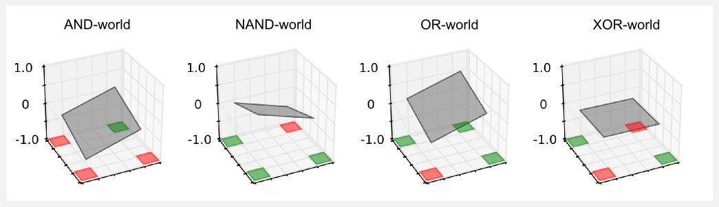
The result is much better! The planes are no more flat, because introducing the bias we gave the possibility to shift up and down. Now the planes can be adjusted to fit all the constraints. The script will also print the weight vector and the utilities returned by this approximator:
------AND-world------
w: [ 0.12578254  0.12194905 -0.71257655]
[[-0.21 -0.09  0.03  0.16  0.28]
 [-0.34 -0.21 -0.09  0.03  0.15]
 [-0.46 -0.34 -0.22 -0.1   0.03]
 [-0.59 -0.46 -0.34 -0.22 -0.1 ]
 [-0.71 -0.59 -0.47 -0.35 -0.22]]

------NAND-world------
w: [-0.12242233 -0.12346582  0.71111163]
[[ 0.22  0.1  -0.03 -0.15 -0.27]
 [ 0.34  0.22  0.1  -0.03 -0.15]
 [ 0.47  0.34  0.22  0.1  -0.03]
 [ 0.59  0.47  0.34  0.22  0.09]
 [ 0.71  0.59  0.46  0.34  0.22]]

------OR-world------
w: [ 0.12406486  0.11832163 -0.26037356]
[[ 0.24  0.35  0.47  0.59  0.71]
 [ 0.11  0.23  0.35  0.47  0.59]
 [-0.01  0.11  0.22  0.34  0.46]
 [-0.14 -0.02  0.1   0.22  0.34]
 [-0.26 -0.14 -0.02  0.09  0.21]]

------XOR-world------
w: [ 0.00220366 -0.00094763  0.00044972]
[[ 0.01  0.01  0.01  0.01  0.01]
 [ 0.01  0.01  0.01  0.    0.  ]
 [ 0.    0.    0.    0.    0.  ]
 [ 0.    0.    0.   -0.   -0.  ]
 [ 0.   -0.   -0.   -0.   -0.  ]]
The utility matrix printed on terminal is obtained computing the output of the linear approximator for each state of the gridworld. In Numpy the state (0,0) is the element in the top left corner and it can be hard to read when printing the matrix. For this reason the matrix has been vertically flipped in order to match the values with the cells of the gridworld. Giving a look to the utilities we can see that in most of the worlds they are pretty good. For instance, in the AND-world we should have an utility of -1.0 for the state (0,0). The approximator returned an utility of -0.71 (bottom-left element in the matrix). On the other two red cells the values are -0.21 and -0.22 which are not so close to -1.0 but are at least negative. The positive cell in state (4,4) has an utility of 1.0 and the approximator returned 0.28.
At this point it should be clear why having a function approximator is a big deal. With the lookup table approach we could represent the utilities of the boolean worlds using a table with 5 rows and 5 columns, for a total of 25 variables to keep in memory. Now we only need two weights and a bias, for a total of 3 variables. Everything seems fine, we have an approximator which works pretty well and is easy to tune. However our problems are not finished. If you look to the XOR-world you will notice that the plane is still flat. This problem is much serious than the previous one and there is no way to solve it. There is no plane that can separate red and green cells in the XOR-world. Try it yourself, adjust the plane to satisfy all the constraints. That is not feasible. The XOR-world is not linearly separable, and using a linear approximator we can only approximate linearly separable functions. The only chance we have to approximate an utility function for the XOR-world is to literally bend the plane, and to do it we have to use an higher order approximator.
High-order approximators
The linear approximator is the simplest form of approximation. The linear case is appealing not only for its simplicity but also because it is guaranteed to converge. However, there is an important limit implicit in the linear model: it cannot represent complex relationships between features. That’s it, the linear form does not allow representing the interaction between features. Such a complex interaction naturally arise in physical systems. Some features may be informative only when other features are absent. For example, the inverted pendulum angular position and velocity are tightly connected. A high angular velocity may be either good or bad depending on the position of the pole. If the angle is high then high angular velocity means an imminent danger of falling, whereas if the angle is low then high angular velocity means the pole is righting itself.
Solving the XOR problem is very easy when an additional feature is added.
\[\hat{U}(s, \boldsymbol{w}) = x_{1} w_{1} + x_{2} w_{2} + x_{1} x_{2} w_{3} + w_{4}\]If you look to the equation what I added is the new term \(x_{1} x_{2} w_{3}\). This term introduces a relationship between the two features \(x_{1}\) and \(x_{2}\). Now the surface represented by the equation is no more a plane but an hyperbolic paraboloid, a saddle-like surface which perfectly adapt to the XOR-world. We do not need to rewrite the update function because it remains unchanged. We always have a linear combination of features and the gradient is always equal to the input vector. In the repository you will find another script called xor_paraboloid.py containing an implementation of this new approximator. Running the script with the same parameters used for the linear case we end up with the following plot:
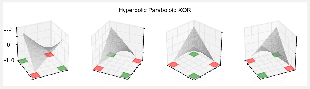
Here the paraboloid is represented using four different perspectives. The result obtained at the end of the training shows that the utilities are very good.
w: [ 0.36834857  0.36628493 -0.18575494 -0.73988694]
[[ 0.73  0.36 -0.02 -0.4  -0.77]
 [ 0.37  0.17 -0.02 -0.21 -0.4 ]
 [-0.   -0.01 -0.01 -0.02 -0.02]
 [-0.37 -0.19 -0.01  0.17  0.35]
 [-0.74 -0.37 -0.01  0.36  0.73]]
We should have -1 in the bottom-left and top-right corners, the approximator returned -0.74 and -0.77 which are pretty good estimations. Similar results have been obtained for the positive states in the top-left and bottom-right corners, where the approximator returned 0.73 and 0.77 which are very close to the true utility of 1.0. I suggest you to run the script using different hyper-parameters (e.g. the learning rate alpha) to see the effects on the final plot and on the utility table.
The geometrical intuition is helpful because it gives an immediate intuition of the different approximators. We saw that using additional features and more complex functions it is possible to better describe the utility space. High-order approximators may find useful links between futures whereas a pure linear approximator could not. An example of high-order approximator is the quadratic approximator. In the quadratic approximator we use a second order polynomial to model the utility function.
\[\hat{U}(s, \boldsymbol{w}) = x_{1} w_{1} + x_{2} w_{2} + x_{1}^{2} w_{3} + x_{2}^{2} w_{4} +... + x_{N-1} w_{M-1} + x_{N}^{2} w_{M}\]It is not easy to choose the right polynomial. A simple approximator like the linear one can miss the relevant relations between features and target, whereas an high order approximator can fail to generalise to new unseen states. The optimal balance is achieved through a delicate tradeoff known in machine learning as the bias-variance tradeoff.
Conclusions
In this post I introduced function approximation and we saw how to build a methodology based on an error measure, an update rule, and a target. This methodology is extremely flexible and we are going to use it again in future posts. Moreover I introduced linear methods, which are the simplest approximators. Linear function approximation is limited because it cannot capture important relationships between features. Using an high-order polynomial can often solve the problem but is still a limited approach because modelling the relationship between features remain a design choice. In complex physical systems multiple elements are interacting and it will be difficult to find the right polynomial that may describe those relationships. How to solve this problem? We can use non-linear function approximators. In the next post I will introduce neural networks and show you how to use it in reinforcement learning.
Index
- [First Post] Markov Decision Process, Bellman Equation, Value iteration and Policy Iteration algorithms.
- [Second Post] Monte Carlo Intuition, Monte Carlo methods, Prediction and Control, Generalised Policy Iteration, Q-function.
- [Third Post] Temporal Differencing intuition, Animal Learning, TD(0), TD(λ) and Eligibility Traces, SARSA, Q-learning.
- [Fourth Post] Neurobiology behind Actor-Critic methods, computational Actor-Critic methods, Actor-only and Critic-only methods.
- [Fifth Post] Evolutionary Algorithms introduction, Genetic Algorithm in Reinforcement Learning, Genetic Algorithms for policy selection.
- [Sixt Post] Reinforcement learning applications, Multi-Armed Bandit, Mountain Car, Inverted Pendulum, Drone landing, Hard problems.
- [Seventh Post] Function approximation, Intuition, Linear approximator, Applications, High-order approximators.
- [Eighth Post] Non-linear function approximation, Perceptron, Multi Layer Perceptron, Applications, Policy Gradient.
Resources
-
The complete code for the Reinforcement Learning Function Approximation is available on the dissecting-reinforcement-learning official repository on GitHub.
-
Reinforcement learning: An introduction (Chapter 8 ‘Generalization and Function Approximation’) Sutton, R. S., & Barto, A. G. (1998). Cambridge: MIT press. [html]
References
Bowers, J. S. (2009). On the biological plausibility of grandmother cells: implications for neural network theories in psychology and neuroscience. Psychological review, 116(1), 220.
Gross, C. G., Rocha-Miranda, C. E. D., & Bender, D. B. (1972). Visual properties of neurons in inferotemporal cortex of the Macaque. Journal of neurophysiology, 35(1), 96-111.
Gross, C. G. (2002). Genealogy of the “grandmother cell”. The Neuroscientist, 8(5), 512-518.
Hinton, G. E. (1984). Distributed representations.
Plaut, D. C., & McClelland, J. L. (2010). Locating object knowledge in the brain: Comment on Bowers’s (2009) attempt to revive the grandmother cell hypothesis.