Dissecting Reinforcement Learning-Part.1
Premise[This post is an introduction to reinforcement learning and it is meant to be the starting point for a reader who already has some machine learning background and is confident with a little bit of math and Python. When I study a new algorithm I always want to understand the underlying mechanisms and implement the algorithm from scratch using a programming language. I followed this approach in this post which can be long to read but worthy.]
When I started to study reinforcement learning I did not find any good online resource which explained from the basis what reinforcement learning really is. Most of the (very good) blogs out there focus on the modern approaches (Deep Reinforcement Learning) and introduce the Bellman equation without a satisfying explanation. I turned my attention to books and I found the one of Russel and Norvig called Artificial Intelligence: A Modern Approach.

This post is based on chapters 17 of the second edition, and it can be considered an extended review of the chapter. I will use the same mathematical notation of the authors, in this way you can use the book to cover some missing parts or vice versa. You can find the complete code used in this post in my github repository, with the PDF version of the post. In the next section I will introduce Markov chains, if you already know this concept you can skip to the next section…
In the beginning was Andrey Markov
Andrey Markov was a Russian mathematician who studied stochastic processes. Markov was particularly interested in systems that follow a chain of linked events. In 1906 Markov produced interesting results about discrete processes that he called chains. A Markov Chain has a set of states \(S = \{ s_0, s_1, ... , s_m \}\) and a process that can move successively from one state to the other. Each move is a single step and is based on a transition model \(T\). You should make some effort in remembering the keywords in bold, we will use them extensively during the rest of the article. To summarise a Markov chain is defined as follows:
- Set of possible States: \(S = \{ s_0, s_1, ... , s_m \}\)
- Initial State: \(s_0\)
- Transition Model: \(T(s, s^{'})\)
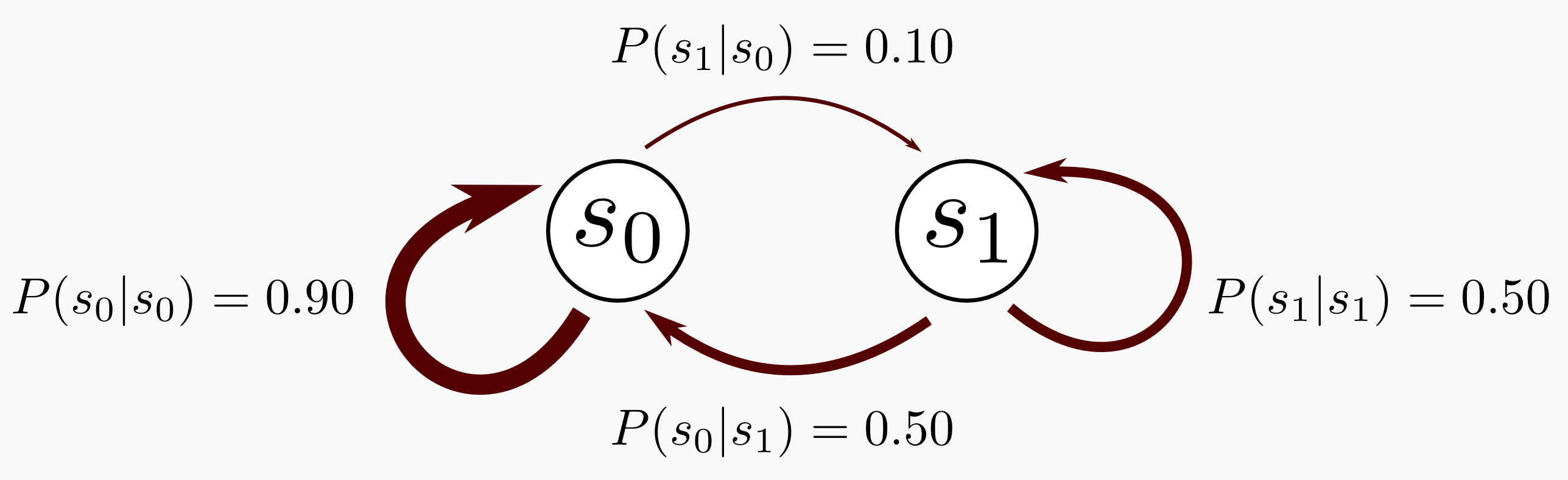
There is something peculiar in a Markov chain that I did not mention. A Markov chain is based on the Markov Property. The Markov property states that given the present, the future is conditionally independent of the past. That’s it, the state in which the process is now it is dependent only from the state it was at \(t-1\). An example can simplify the digestion of Markov chains. Let’s suppose we have a chain with only two states \(s_0\) and \(s_1\), where \(s_0\) is the initial state. The process is in \(s_0\) 90% of the time and it can move to \(s_1\) the remaining 10% of the time. When the process is in state \(s_1\) it will remain there 50% of the time. Given this data we can create a Transition Matrix \(T\) as follow:
\[T = \begin{bmatrix} 0.90 & 0.10 \\ 0.50 & 0.50 \end{bmatrix}\]The transition matrix is always a square matrix, and since we are dealing with probability distributions all the entries are within 0 and 1 and a single row sums to 1. We can graphically represent the Markov chain. In the following representation each state of the chain is a node and the transition probabilities are edges. Highest probabilities have a thickest edge:
Until now we did not mention time, but we have to do it because Markov chains are dynamical processes which evolve in time. Let’s suppose we have to guess were the process will be after 3 steps and after 50 steps. How can we do it? We are interested in chains that have a finite number of states and are time-homogeneous meaning that the transition matrix does not change over time. Given these assumptions we can compute the k-step transition probability as the k-th power of the transition matrix, let’s do it in Numpy:
import numpy as np

#Declaring the Transition Matrix T
T = np.array([[0.90, 0.10],
              [0.50, 0.50]])

#Obtaining T after 3 steps
T_3 = np.linalg.matrix_power(T, 3)
#Obtaining T after 50 steps
T_50 = np.linalg.matrix_power(T, 50)
#Obtaining T after 100 steps
T_100 = np.linalg.matrix_power(T, 100)

#Printing the matrices
print("T: " + str(T))
print("T_3: " + str(T_3))
print("T_50: " + str(T_50))
print("T_100: " + str(T_100))
T: [[ 0.9  0.1]
    [ 0.5  0.5]]

T_3: [[ 0.844  0.156]
      [ 0.78   0.22 ]]

T_50: [[ 0.83333333  0.16666667]
       [ 0.83333333  0.16666667]]

T_100: [[ 0.83333333  0.16666667]
        [ 0.83333333  0.16666667]]
Now we define the initial distribution which represent the state of the system at k=0. Our system is composed of two states and we can model the initial distribution as a vector with two elements, the first element of the vector represents the probability of staying in state \(s_0\) and the second element the probability of staying in state \(s_1\). Let’s suppose that we start from \(s_0\), the vector \(\mathbf{v}\) representing the initial distribution will have the form
\[\mathbf{v} = (1, 0)\]We can calculate the probability of being in a specific state after k iterations multiplying the initial distribution and the transition matrix: \(\mathbf{v} \cdot T^{k}\). Let’s do it in Numpy:
import numpy as np

#Declaring the initial distribution
v = np.array([[1.0, 0.0]])
#Declaring the Transition Matrix T
T = np.array([[0.90, 0.10],
              [0.50, 0.50]])

#Obtaining T after 3 steps
T_3 = np.linalg.matrix_power(T, 3)
#Obtaining T after 50 steps
T_50 = np.linalg.matrix_power(T, 50)
#Obtaining T after 100 steps
T_100 = np.linalg.matrix_power(T, 100)

#Printing the initial distribution
print("v: " + str(v))
print("v_1: " + str(np.dot(v,T)))
print("v_3: " + str(np.dot(v,T_3)))
print("v_50: " + str(np.dot(v,T_50)))
print("v_100: " + str(np.dot(v,T_100)))
v: [[ 1.  0.]]

v_1: [[ 0.9  0.1]]

v_3: [[ 0.844  0.156]]

v_50: [[ 0.83333333  0.16666667]]

v_100: [[ 0.83333333  0.16666667]]
What’s going on? The process starts at \(s_0\) and after one iteration we can be 90% sure it is still in that state. This is easy to grasp, our transition model says that the process can stay in \(s_0\) with 90% probability, nothing new. Looking to the state distribution at k=3 we notice that there is something different. We are moving in the future and different branches are possible. If we want to find the probability of being in state \(s_0\) after three iteration we should sum all the possible branches that lead to \(s_0\). A picture is worth a thousand words:
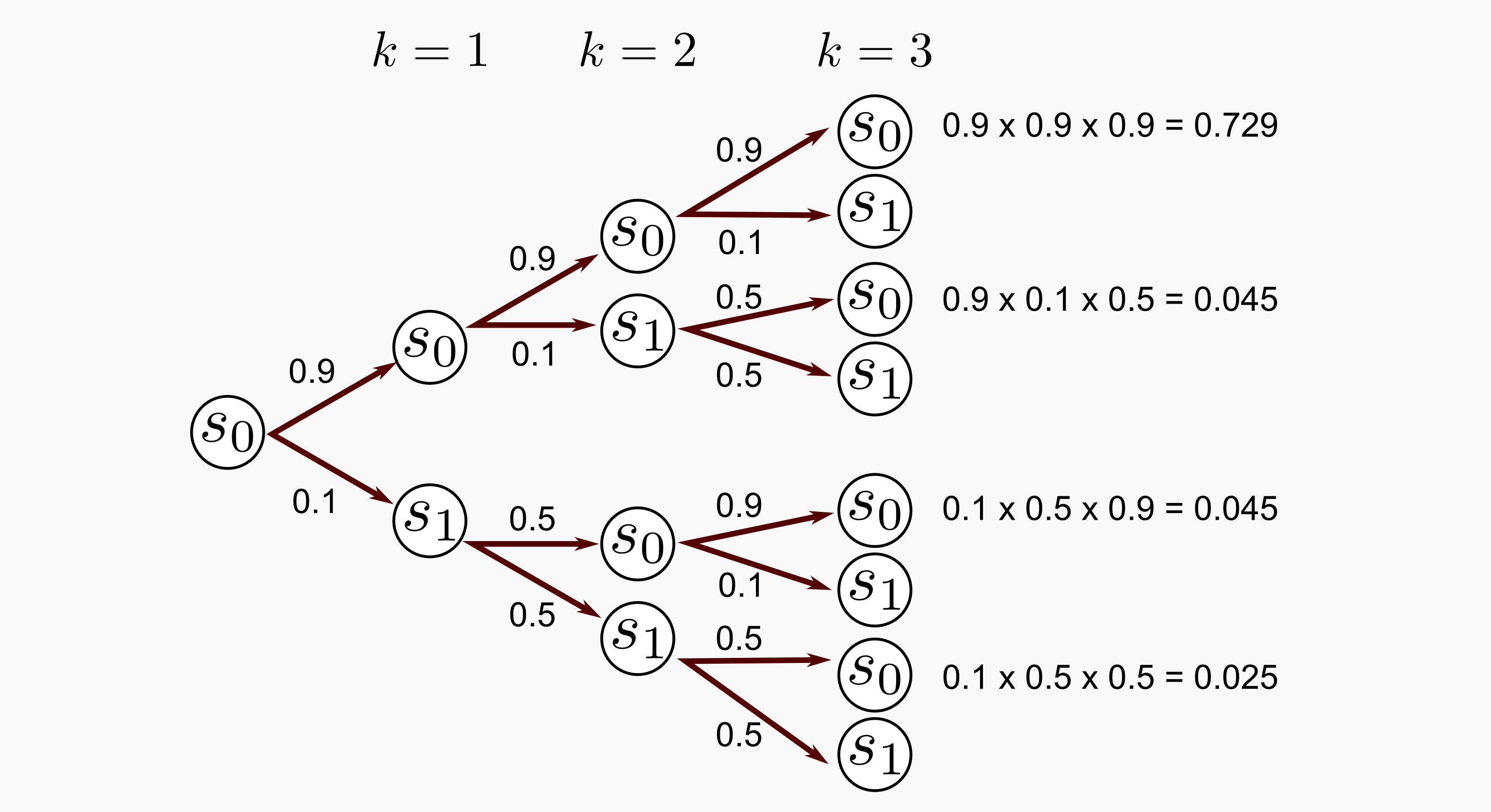
The possibility to be in \(s_0\) at \(k=3\) is given by (0.729 + 0.045 + 0.045 + 0.025) which is equal to 0.844 we got the same result. Now let’s suppose that at the beginning we have some uncertainty about the starting state of our process, let’s define another starting vector as follows:
\[\mathbf{v} = (0.5, 0.5)\]That’s it, with a probability of 50% we can start from \(s_0\). Running again the Python script we print the results after 1, 3, 50 and 100 iterations:
v: [[ 0.5, 0.5]]

v_1: [[ 0.7  0.3]]

v_3: [[ 0.812  0.188]]

v_50: [[ 0.83333333  0.16666667]]

v_100: [[ 0.83333333  0.16666667]]
This time the probability of being in \(s_0\) at k=3 is lower (0.812), but in the long run we have the same outcome (0.8333333). What is happening in the long run? The result after 50 and 100 iterations are the same and v_50 is equal to v_100 no matter which starting distribution we have. The chain converged to equilibrium meaning that as the time progresses it forgets about the starting distribution. But we have to be careful, the convergence is not always guaranteed. The dynamics of a Markov chain can be very complex, in particular it is possible to have transient and recurrent states. For our scope what we saw is enough. I suggest you to give a look at the setosa.io blog because they have an interactive page for Markov chain visualization.
Markov Decision Process
In reinforcement learning it is used a concept that is affine to Markov chains, I am talking about Markov Decision Processes (MDPs). A MDP is a reinterpretation of Markov chains which includes an agent and a decision making stage. A MDP is defined by these components:
- Set of possible States: \(S = \{ s_0, s_1, ..., s_m \}\)
- Initial State: \(s_0\)
- Set of possible Actions: \(A = \{ a_0, a_1, ..., a_n \}\)
- Transition Model: \(T(s, a, s^{'})\)
- Reward Function: \(R(s)\)
As you can see we are introducing some new elements compared to Markov chains. The transition model depends on the current state, the next state and the action of the agent. The transition model returns the probability of reaching the state \(s^{'}\) if the action \(a\) is done in state \(s\). But given \(s\) and \(a\) the model is conditionally independent of all previous states and actions (Markov Property). Moreover there is the Reward function \(R(s)\) which return a real value every time the agent moves from one state to the other (Attention: defining the Reward function to depend only from \(s\) can be confusing, Russel and Norvig used this notation in the book to simplify the description, it does not change the problem in any significant way). Since we have a reward function we can say that some states are more desirable that others because when the agent moves in those states it receives a higher reward. On the opposite there are states that are not desirable at all, because when the agent moves there it receives a negative reward.
-
Problem the agent has to maximise the reward avoiding states that return negative values and choosing the one that return positive values.
-
Solution find a policy \(\pi(s)\) that returns the action with the highest reward.
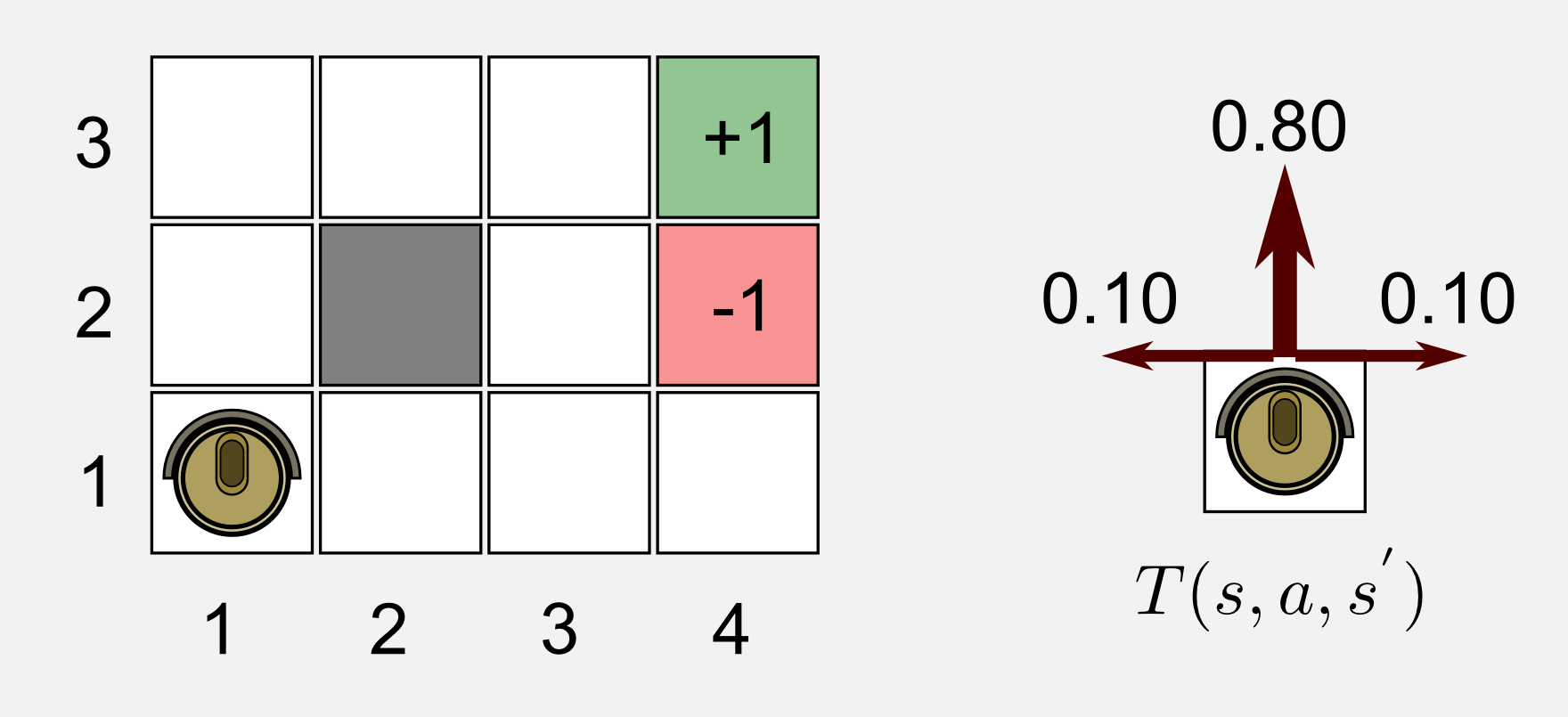
The agent can try different policies but only one of those can be considered an optimal policy, denoted by \(\pi^{*}\), which yields to the highest expected utility. It is time to introduce an example that I am going to use along all the post. This example is inspired by the simple environment presented by Russel and Norving in chapter 17.1 of their book. Let suppose we have a cleaning robot that has to reach a charging station. Our simple world is a 4x3 matrix where the starting point \(s_0\) is at (1,1), the charging station at (4,3), dangerous stairs at (4,2), and an obstacle at (2,2). The robot has to find the best way to reach the charging station (Reward +1) and to avoid falling down the flight of stairs (Reward -1). Every time the robot takes a decision it is possible to have the interference of a stochastic factor (ex. the ground is slippery, an evil cat is stinging the robot), which makes the robot diverge from the original path 20% of the time. If the robot decides to go ahead in 10% of the cases it will finish on the left and in 10% of the cases on the right state. If the robot hits the wall or the obstacle it will bounce back to the previous position. The main characteristics of this world are the following:
- Discrete time and space
- Fully observable
- Infinite horizon
- Known Transition Model
The environment is fully observable, meaning that the robot always knows in which state it is in. The infinite horizon clause should be explained further. Infinite horizon means that there is not a fixed time limit. If the agent has a policy for going back an forth in the same two states, it will go on forever. This assumption does not mean that in every episode the agent has to pass for a series of infinite states. When one of the two terminal states is reached, the episode stops. A representation of this world and the transition model are reported below. Be careful with the indexing used by Russell and Norvig, it can be confusing. They named each state of the world by the column and row, starting from the bottom-left corner.
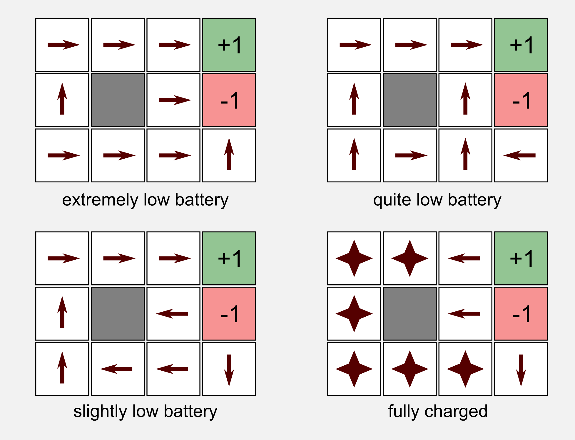
I said that the aim of the robot is to find the best way to reach the charging station, but what does it mean the best way? Depending on the type of reward the robot is receiving for each intermediate state we can have different optimal policies \(\pi^{*}\). Let’s suppose we are programming the firmware of the robot. Based on the battery level we give a different reward at each time step. The rewards for the two terminal states remain the same (charger=+1, stairs=-1). The obstacle at (2,2) is not a valid state and therefore there is no reward associated to it. Given these assumptions we can have four different cases:
- \(R(s) \leq -1.6284\) extremely low battery
- \(-0.4278 \leq R(s) \leq -0.085\) quite low battery
- \(-0.0221 \leq R(s) \leq 0\) slightly low battery
- \(R(s) > 0\) fully charged
For each one of these conditions we can try to guess which policy the agent will choose. In the extremely low battery scenario the agent receives such a high punishment that it only wants to stop the pain as soon as possible. Life is so painful that falling down the flight of stairs is a good choice. In the quite low battery scenario the agent takes the shortest path to the charging station, it does not care about falling down. In the slightly low battery case the robot does not take risks at all and it avoids the stairs at cost of banging against the wall. Finally in the fully charged case the agent remains in a steady state receiving a positive reward at each time step.
Until now we know the kind of policies that can emerge in specific environments with defined rewards, but there is still something I did not talk about: how can the agent choose the best policy?
The Bellman equation
The previous section finished with a question: how can the agent choose the best policy? To give an answer to this question I will present the Bellman equation. First of all we have to find a way to compare two policies. We can use the reward given at each state to obtain a measure of the utility of a state sequence. We define the utility of the states history \(h\) as:
\[U_{h} = R(s_0) + \gamma R(s_1) + \gamma^{2} R(s_2) + ... + \gamma^{n} R(s_n)\]The previous formula defines the Discounted Rewards of a state sequence, where \(\gamma \in [0,1]\) is called the discount factor. The discount factor describes the preference of the agent for the current rewards over future rewards. A discount factor of 1.0 collapses the previous formula into additive rewards. The discounted rewards are not the only way we can estimate the utility, but it is the one giving less problems. For example, in the case of an infinite sequence of states the discounted reward gives a finite utility (using the sum of infinite series), moreover we can also compare infinite sequences using the average reward obtained per time step. How to compare the utility of single states? The utility \(U(s)\) can be defined as:
\[U(s) = E\bigg[ \sum_{t=0}^{\infty} \gamma^t R(s_t) \bigg]\]Let’s recall that the utility is defined with respect of a policy \(\pi\) which for simplicity I did not mention. Once we have the utilities, how can we choose the best action for the next state? Using the maximum expected utility principle which says that a rational agent should choose an action that maximise its expected utility. We are a step closer to the Bellman equation. What we miss is to recall that the utility of a state \(s\) is correlated with the utility of its neighbours at \(s^{'}\), meaning:
\[U(s) = R(s) + \gamma \underset{a}{\text{ max }} \sum_{s^{'}}^{} T(s,a,s^{'}) U(s^{'})\]We just derived the Bellman equation! Using the Bellman equation an agent can estimate the best action to take and find the optimal policy. Let’s try to dissect this equation. First, the term \(R(s)\) is something we have to add for sure in the equation. We are in state \(s\) and we know the reward given for that state, the utility must take it into account. Second, notice that the equation is using the transition model \(T\) which is multiplied by the utility of the next state \(s^{'}\). If you think about that it makes sense, a state which has a low probability to happen (like the 10% probability of moving on the left and on the right in our simplified world) will have a lowest weight in the summation.
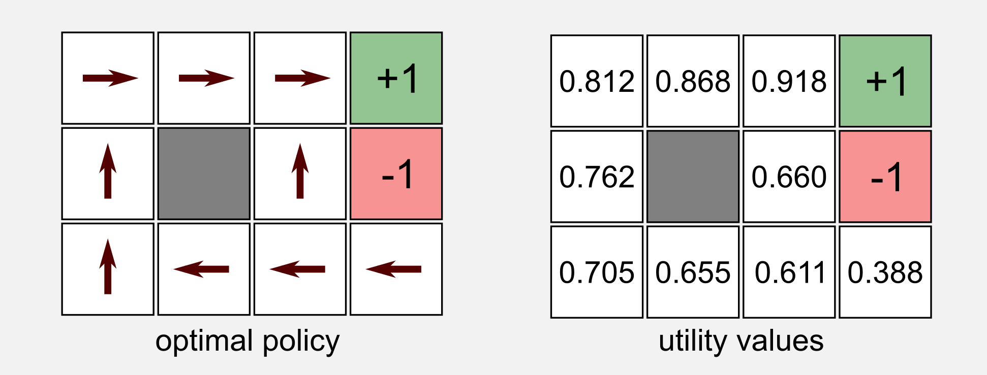
To empirically test the Bellman equation we are going to use our cleaning robot in the simplified 4x3 environment. In this example the reward for each non-terminal state is \(R(s) = -0.04\). We can imagine to have the utility values for each one of the states, for the moment you do not need to know how we got these values, imagine they appeared magically. In the same magical way we obtained the optimal policy for the world (to double-check if what we will obtain from the Bellman equation makes sense). This image is very important, keep it in mind.
In our example we suppose the robot starts from the state (1,1). Using the Bellman equation we have to find the action with the highest utility between UP, LEFT, DOWN and RIGHT. We do not have the optimal policy, but we have the transition model and the utility values for each state. You have to recall the two main rules of our environment: (i) if the robot bounce on the wall it goes back to the previous state, and (ii) the selected action is executed only with a probability of 80% in accordance with the transition model. Instead of dealing with those ugly numbers I want to show you a visual representaion of the possible outcomes:
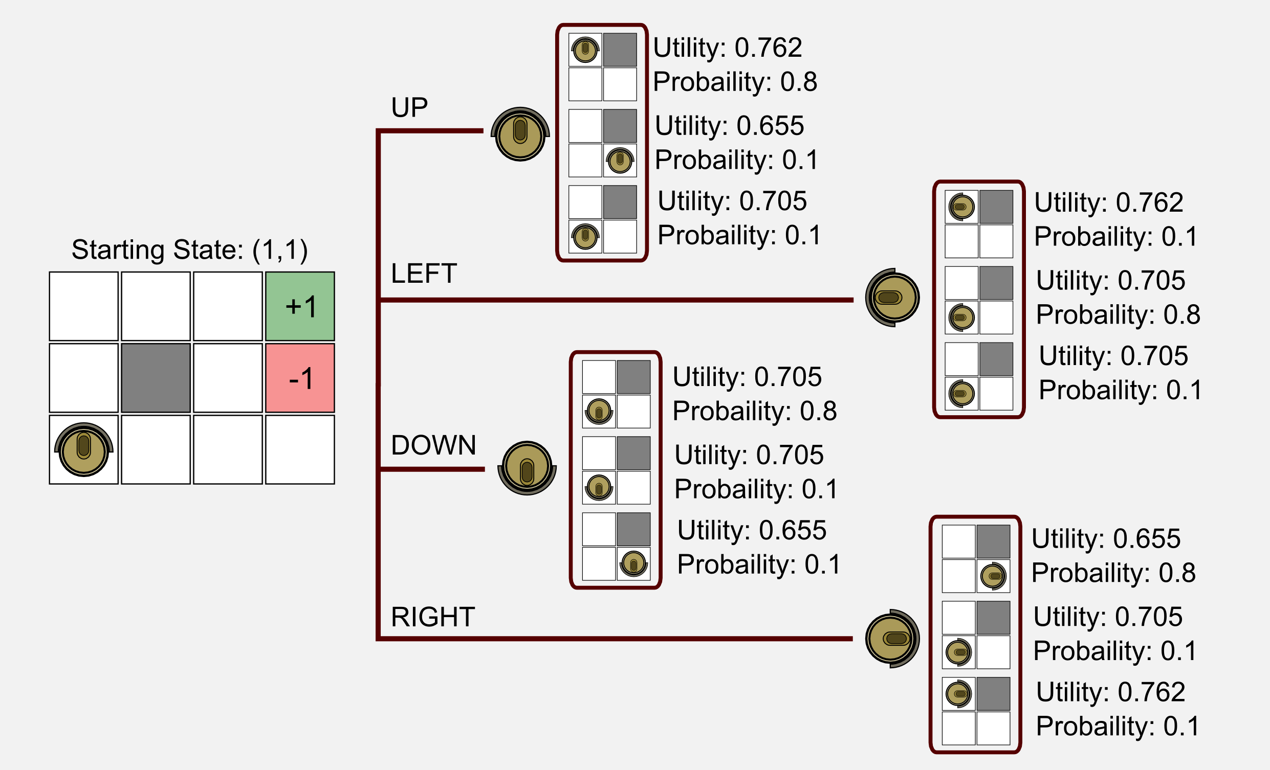
For each possible outcome I reported the utility and the probability given by the transition model. This corresponds to the first part of the Bellman equation. The next step is to calculate the product between the utility and the transition probability, then sum up the value for each action.
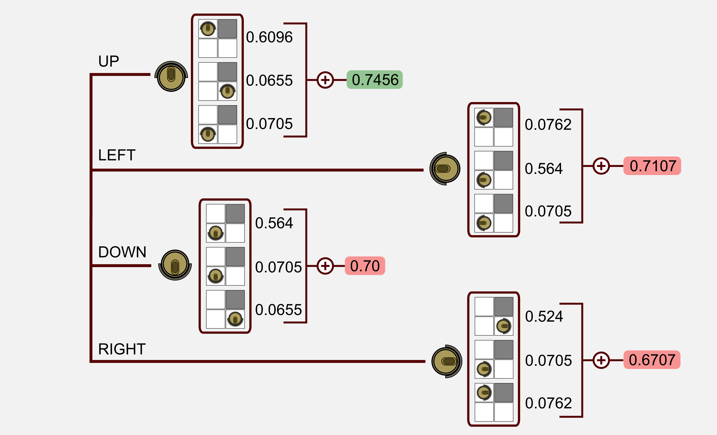
We found out that for state (1,1) the action UP has the highest value. This is in accordance with the optimal policy we magically got. This part of the Bellman equation returns the action that maximizes the expected utility of the subsequent state, which is what an optimal policy should do:
\[\pi^{*}(s) = \underset{a}{\text{ argmax }} \sum_{s^{'}}^{} T(s,a,s^{'}) U(s^{'})\]Now we have all the elements and we can plug the values in the Bellman equation finding the utility of the state (1,1):
\[U(s_{11}) = -0.04 + 1.0 \times 0.7456 = 0.7056\]The Bellman equation works! What we need is a Python implementation of the equation to use in our simulated world. We are going to use the same terminology of the previous sections. Our world has 4x3=12 possible states. The starting vector contains 12 values and the transition matrix is a huge 12x12x4 matrix (12 starting states, 12 next states, 4 actions) where most of the values are zeros (we can move only from one state to its neighbours). I generated the transition matrix using a script and I saved it as a Numpy matrix (you can download it here).
In the script I defined the function return_state_utility() which is an implementation of the Bellman equation. Using this function we are going to print the utility of the state (1,1) and check if it is the same we found previously:
import numpy as np

def return_state_utility(v, T, u, reward, gamma):
    """Return the state utility.

    @param v the state vector
    @param T transition matrix
    @param u utility vector
    @param reward for that state
    @param gamma discount factor
    @return the utility of the state
    """
    action_array = np.zeros(4)
    for action in range(0, 4):
        action_array[action] = np.sum(np.multiply(u, np.dot(v, T[:,:,action])))
    return reward + gamma * np.max(action_array)

def main():
    #Starting state vector
    #The agent starts from (1, 1)
    v = np.array([[0.0, 0.0, 0.0, 0.0,
                   0.0, 0.0, 0.0, 0.0,
                   1.0, 0.0, 0.0, 0.0]])

    #Transition matrix loaded from file
    #(It is too big to write here)
    T = np.load("T.npy")

    #Utility vector
    u = np.array([[0.812, 0.868, 0.918,   1.0,
                   0.762,   0.0, 0.660,  -1.0,
                   0.705, 0.655, 0.611, 0.388]])

    #Defining the reward for state (1,1)
    reward = -0.04
    #Assuming that the discount factor is equal to 1.0
    gamma = 1.0

    #Use the Bellman equation to find the utility of state (1,1)
    utility_11 = return_state_utility(v, T, u, reward, gamma)
    print("Utility of state (1,1): " + str(utility_11))

if __name__ == "__main__":
    main()
Utility of state (1,1): 0.7056
That’s great, we obtained exactly the same value! Until now we supposed that the utility values appeared magically. Instead of using a magician we want to find an algorithm to obtain these values. There is a problem. For \(n\) possible states there are \(n\) Bellman equations, and each equation contains \(n\) unknowns. Using any linear algebra package would be possible to solve these equations, the problem is that they are not linear because of the \(\text{max}\) operator. What to do? We can use the value iteration algorithm…
The value iteration algorithm
The Bellman equation is the core of the value iteration algorithm for solving a MDP. Our objective is to find the utility (also called value) for each state. As we said we cannot use a linear algebra library, we need an iterative approach. We start with arbitrary initial utility values (usually zeros). Then we calculate the utility of a state using the Bellman equation and we assign it to the state. This iteration is called Bellman update. Applying the Bellman update infinitely often we are guaranteed to reach an equilibrium. Once we reached the equilibrium we have the utility values we were looking for and we can use them to estimate which is the best move for each state. How do we understand when the algorithm reaches the equilibrium? We need a stopping criteria. Taking into account the utilities between two consecutive iterations we can stop the algorithm when no state’s utility changes by much.
\[|| U_{k+1} - U_{k} || < \epsilon \frac{1-\gamma}{\gamma}\]This result is a consequence of the contraction property which I will skip because it is well explained in the chapter 17.2 of the book.
Ok, it’s time to implement the algorithm in Python. I will reuse the return_state_utility() function to update the utility vector u.
import numpy as np

def return_state_utility(v, T, u, reward, gamma):
    """Return the state utility.

    @param v the state vector
    @param T transition matrix
    @param u utility vector
    @param reward for that state
    @param gamma discount factor
    @return the utility of the state
    """
    action_array = np.zeros(4)
    for action in range(0, 4):
        action_array[action] = np.sum(np.multiply(u, np.dot(v, T[:,:,action])))
    return reward + gamma * np.max(action_array)

def main():
    #Change as you want
    tot_states = 12
    gamma = 0.999 #Discount factor
    iteration = 0 #Iteration counter
    epsilon = 0.01 #Stopping criteria small value

    #List containing the data for each iteation
    graph_list = list()

    #Transition matrix loaded from file (It is too big to write here)
    T = np.load("T.npy")

    #Reward vector
    r = np.array([-0.04, -0.04, -0.04,  +1.0,
                  -0.04,   0.0, -0.04,  -1.0,
                  -0.04, -0.04, -0.04, -0.04])

    #Utility vectors
    u = np.array([0.0, 0.0, 0.0,  0.0,
                   0.0, 0.0, 0.0,  0.0,
                   0.0, 0.0, 0.0,  0.0])
    u1 = np.array([0.0, 0.0, 0.0,  0.0,
                    0.0, 0.0, 0.0,  0.0,
                    0.0, 0.0, 0.0,  0.0])

    while True:
        delta = 0
        u = u1.copy()
        iteration += 1
        graph_list.append(u)
        for s in range(tot_states):
            reward = r[s]
            v = np.zeros((1,tot_states))
            v[0,s] = 1.0
            u1[s] = return_state_utility(v, T, u, reward, gamma)
            delta = max(delta, np.abs(u1[s] - u[s])) #Stopping criteria
        if delta < epsilon * (1 - gamma) / gamma:
                print("=================== FINAL RESULT ==================")
                print("Iterations: " + str(iteration))
                print("Delta: " + str(delta))
                print("Gamma: " + str(gamma))
                print("Epsilon: " + str(epsilon))
                print("===================================================")
                print(u[0:4])
                print(u[4:8])
                print(u[8:12])
                print("===================================================")
                break

if __name__ == "__main__":
    main()
It is interesting to give a look at the stabilization of each utility during the convergence. Using matplotlib I draw the utility value of each state for 25 iterations.
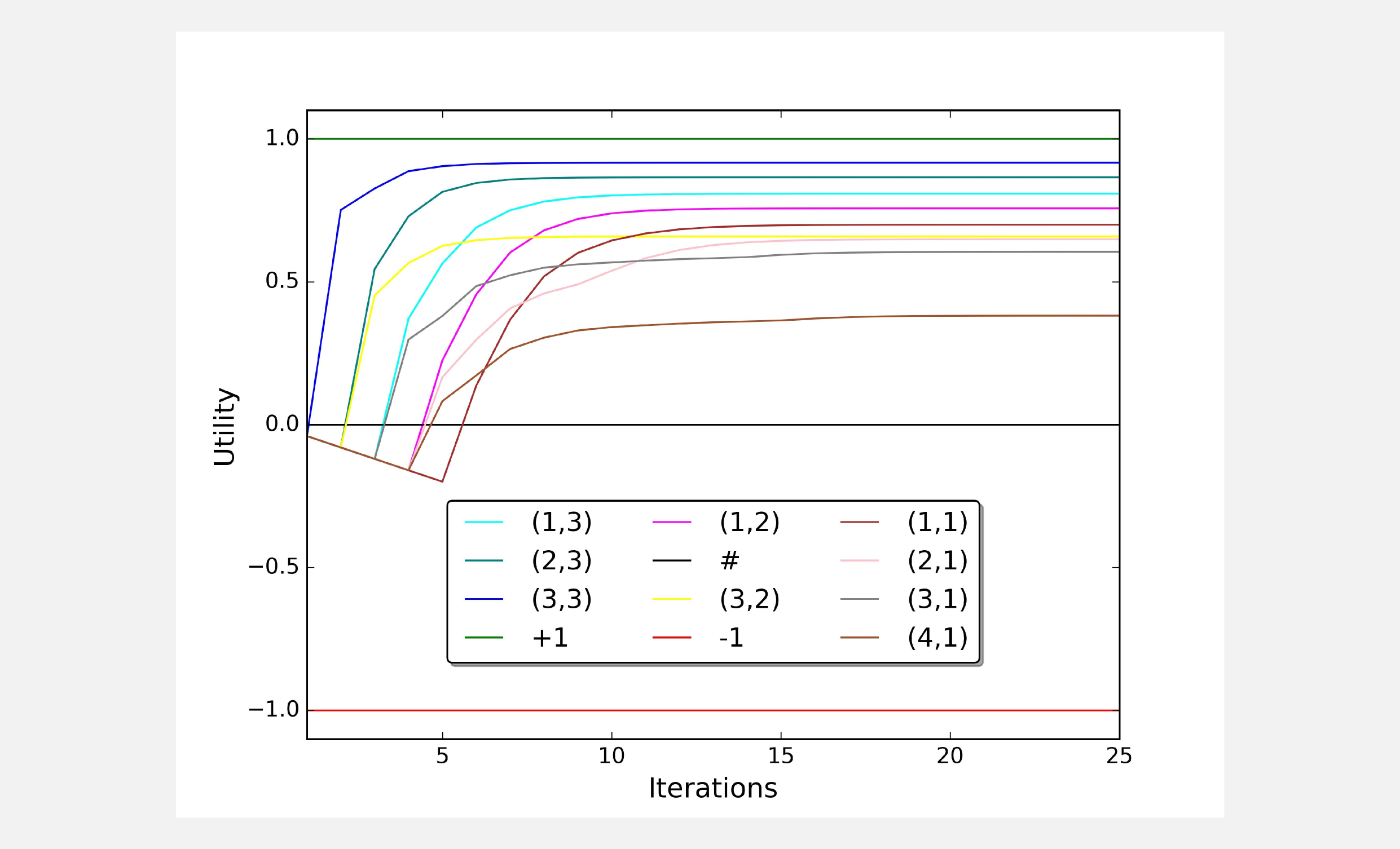
Using the same code I run different simulations with different values for the discounting factor gamma. When the discounting factor approaches 1.0 our prediction for the utilities gets more precise. In the limit case of gamma = 1.0 the algorithm will never end because we will never reach the stopping criteria.
=================== FINAL RESULT ==================
Iterations: 9
Delta: 0.000304045
Gamma: 0.5
Epsilon: 0.001
===================================================
[[ 0.00854086  0.12551955  0.38243452  1.        ]]
[[-0.04081336  0.          0.06628399 -1.        ]]
[[-0.06241921 -0.05337728 -0.01991461 -0.07463402]]
===================================================
=================== FINAL RESULT ==================
Iterations: 16
Delta: 0.000104779638547
Gamma: 0.9
Epsilon: 0.001
===================================================
[[ 0.50939438  0.64958568  0.79536209  1.        ]]
[[ 0.39844322  0.          0.48644002 -1.        ]]
[[ 0.29628832  0.253867    0.34475423  0.12987275]]
===================================================
=================== FINAL RESULT ==================
Iterations: 29
Delta: 9.97973302774e-07
Gamma: 0.999
Epsilon: 0.001
===================================================
[[ 0.80796344  0.86539911  0.91653199  1.        ]]
[[ 0.75696623  0.          0.65836281 -1.        ]]
[[ 0.69968285  0.64882069  0.6047189   0.38150244]]
===================================================
There is another algorithm that allows us to find the utility vector and at the same time an optimal policy, the policy iteration algorithm.
The policy iteration algorithm
With the value iteration algorithm we have a way to estimate the utility of each state. What we still miss is a way to estimate an optimal policy. In this section, I am going to show you how we can use the policy iteration algorithm to find an optimal policy that maximizes the expected reward. No policy generates more reward than the optimal policy \(\pi^{*}\). Policy iteration is guaranteed to converge and at convergence, the current policy and its utility function are the optimal policy and the optimal utility function.
First of all, we define a policy \(\pi\) assigning an action to each state. We can assign random actions to this policy, it does not matter. Using the return_state_utility() function (the Bellman equation) we can compute the expected utility of the policy. There is a good news. We do not really need the complete version of the Bellman equation which is:
Since we have a policy and the policy associate to each state an action, we can get rid of the \(\text{ max }\) operator and use a simplified version of the Bellman equation:
\[U(s) = R(s) + \gamma \sum_{s^{'}}^{} T(s,\pi(s),s^{'}) U(s^{'})\]Once we have evaluated the policy, we can improve it. Policy improvement is the second and last step of the algorithm. Our environment has a finite number of states, therefore a finite number of policies. Each iteration returns a better policy. I have implemented a function called return_policy_evaluation() containing the simplified version of the Bellman equation. Moreover, we need the function return_expected_action() returning the action with the highest utility based on the current value of u and T. To check what’s going on I created also a print function, that maps each action contained in the policy vector p to a symbol and print it on terminal.
import numpy as np

def return_policy_evaluation(p, u, r, T, gamma):
  """Return the policy utility.

  @param p policy vector
  @param u utility vector
  @param r reward vector
  @param T transition matrix
  @param gamma discount factor
  @return the utility vector u
  """
  for s in range(12):
    if not np.isnan(p[s]):
      v = np.zeros((1,12))
      v[0,s] = 1.0
      action = int(p[s])
      u[s] = r[s] + gamma * np.sum(np.multiply(u, np.dot(v, T[:,:,action])))
  return u

def return_expected_action(u, T, v):
    """Return the expected action.

    It returns an action based on the
    expected utility of doing a in state s,
    according to T and u. This action is
    the one that maximize the expected
    utility.
    @param u utility vector
    @param T transition matrix
    @param v starting vector
    @return expected action (int)
    """
    actions_array = np.zeros(4)
    for action in range(4):
       #Expected utility of doing a in state s, according to T and u.
       actions_array[action] = np.sum(np.multiply(u, np.dot(v, T[:,:,action])))
    return np.argmax(actions_array)

def print_policy(p, shape):
    """Printing utility.

    Print the policy actions using symbols:
    ^, v, <, > up, down, left, right
    * terminal states
    # obstacles
    """
    counter = 0
    policy_string = ""
    for row in range(shape[0]):
        for col in range(shape[1]):
            if(p[counter] == -1): policy_string += " *  "
            elif(p[counter] == 0): policy_string += " ^  "
            elif(p[counter] == 1): policy_string += " <  "
            elif(p[counter] == 2): policy_string += " v  "
            elif(p[counter] == 3): policy_string += " >  "
            elif(np.isnan(p[counter])): policy_string += " #  "
            counter += 1
        policy_string += '\n'
    print(policy_string)
Now I am going to use these functions in a main loop that is an implementation of the policy iteration algorithm. I declared a new vector p containing the actions for each state. The stopping condition of the algorithm is the difference between the utility vectors after two consecutive iterations. The algorithm terminates when the improvement step has no effect (or a very small effect) over the utilities.
def main():
    gamma = 0.999
    epsilon = 0.0001
    iteration = 0
    T = np.load("T.npy")
    #Generate the first policy randomly
    # NaN=Nothing, -1=Terminal, 0=Up, 1=Left, 2=Down, 3=Right
    p = np.random.randint(0, 4, size=(12)).astype(np.float32)
    p[5] = np.NaN
    p[3] = p[7] = -1
    #Utility vectors
    u = np.array([0.0, 0.0, 0.0,  0.0,
                  0.0, 0.0, 0.0,  0.0,
                  0.0, 0.0, 0.0,  0.0])
    #Reward vector
    r = np.array([-0.04, -0.04, -0.04,  +1.0,
                  -0.04,   0.0, -0.04,  -1.0,
                  -0.04, -0.04, -0.04, -0.04])

    while True:
        iteration += 1
        #1- Policy evaluation
        u_0 = u.copy()
        u = return_policy_evaluation(p, u, r, T, gamma)
        #Stopping criteria
        delta = np.absolute(u - u_0).max()
        if delta < epsilon * (1 - gamma) / gamma: break
        for s in range(12):
            if not np.isnan(p[s]) and not p[s]==-1:
                v = np.zeros((1,12))
                v[0,s] = 1.0
                #2- Policy improvement
                a = return_expected_action(u, T, v)
                if a != p[s]: p[s] = a
        print_policy(p, shape=(3,4))

    print("=================== FINAL RESULT ==================")
    print("Iterations: " + str(iteration))
    print("Delta: " + str(delta))
    print("Gamma: " + str(gamma))
    print("Epsilon: " + str(epsilon))
    print("===================================================")
    print(u[0:4])
    print(u[4:8])
    print(u[8:12])
    print("===================================================")
    print_policy(p, shape=(3,4))
    print("===================================================")

if __name__ == "__main__":
    main()
Running the script with gamma=0.999 and epsilon=0.0001 we get convergence in 22 iterations with the following result:
=================== FINAL RESULT ==================
Iterations: 22
Delta: 9.03617490833e-08
Gamma: 0.999
Epsilon: 0.0001
===================================================
[ 0.80796344  0.86539911  0.91653199  1.        ]
[ 0.75696624  0.          0.65836281 -1.        ]
[ 0.69968295  0.64882105  0.60471972  0.38150427]
===================================================
 >   >   >   *
 ^   #   ^   *
 ^   <   <   <
===================================================
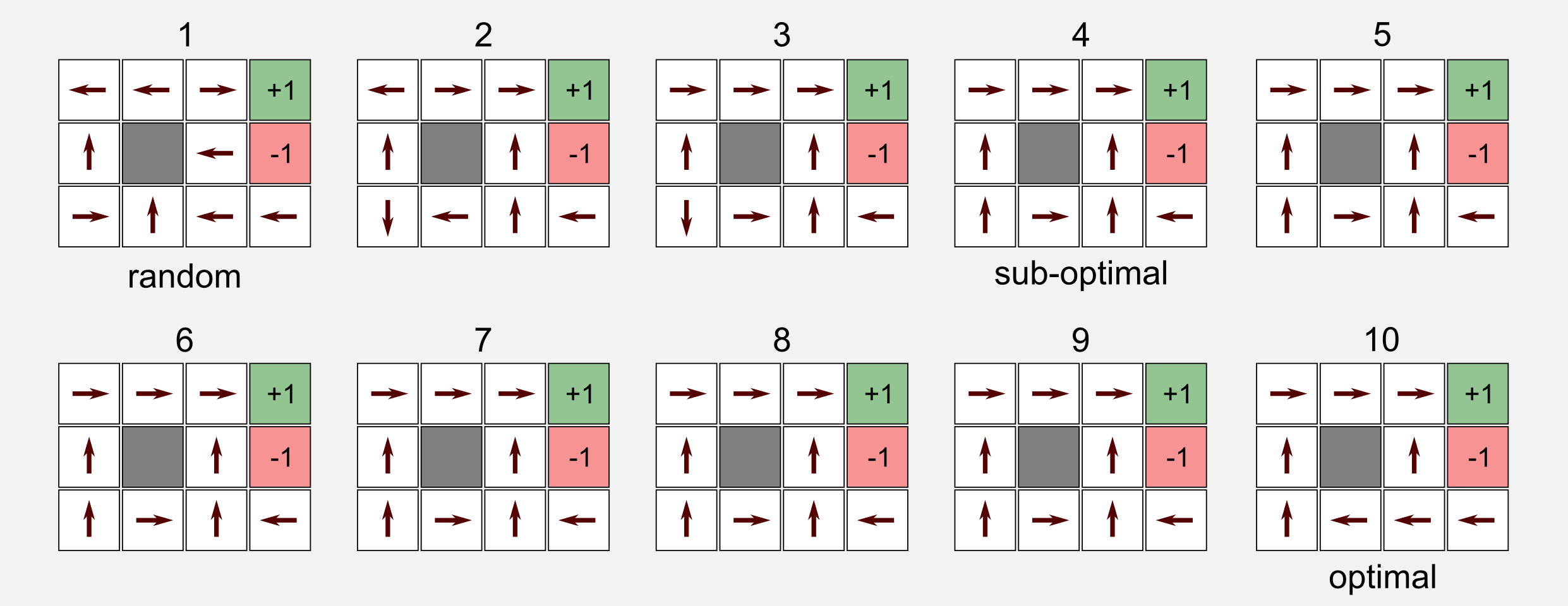
The final policy returned by the algorithm is equal to the optimal policy. Moreover using the simplified Bellman equation the algorithm managed to find good values for the utility vector. If we give a look to the policy evolution we will notice something interesting. At the beginning the policy is randomly generated. After four iterations the algorithm finds a sub-optimal policy and sticks to it until iteration 10 when it finds the optimal policy. From iteration 10 until iteration 22 the algorithm does not change the policy at all. A sub-optimal policy can be a problem in model-free reinforcement learning, because greedy agents can stick to it, but for the moment it is not a problem for us.
Policy iteration and value iteration, which is best? If you have many actions or you start from a fair policy then choose policy iteration. If you have few actions and the transition is acyclic then chose value iteration. If you want the best from the two world then give a look to the modified policy iteration algorithm.
Policy evaluation using linear algebra
I said that eliminating the \(max\) operator from the Bellman equation made our life easier because we could use any linear algebra package to calculate the utilities. In the last section I would like to show you how to reach the same conclusion using a linear algebra approach. In the Bellman equation we have a linear system with \(n\) variables and \(n\) constraints. Remember that here we are dealing with matrices and vectors. Given a policy p and the action associated to the state s, the reward vector r, the transition matrix T and the discount factor gamma, we can estimate the utility in a single line of code:
u[s] = np.linalg.solve(np.identity(12) - gamma*T[:,:,p[s]], r)[s]
I used the Numpy method np.linalg.solve() that takes as input the coefficient matrix A and an array of dependent values b, finding (if it exists) the exact solution to a system of linear equations. If the solution does not exist (e.g. the matrix is not square, or the row-columns are not linearly independent), it is necessary to use the least-squares approximation via the method np.linalg.lstsq().
In both cases we get the solution to the system A x = b. For the matrix A we pass the difference between an identity matrix I and gamma * T, for the dependent array b we pass the reward vector r. Why we pass as first parameter I - gamma*T ? We can derive this value starting from the simplified Bellman equation:
In fact, we could obtain u implementing the last equation in Numpy:
u[s] = np.dot(np.linalg.inv(np.identity(12) - gamma*T[:,:,p[s]]), r)[s]
If you want to use the last expression when an exact solution does not exist, you need to invert the matrix using the pseudoinverse and the Numpy method np.linalg.pinv(). In the end, I prefer to use np.linalg.solve() or np.linalg.lstsq() that does the same thing but is much more readable.
Conclusions
In this first part I summarised the fundamental ideas behind Reinforcement learning. As an example, I used a finite environment with a predefined transition model. What happen if we do not have the transition model? In the next post I will introduce model-free reinforcement learning, that gives an answer to this question with a new set of interesting tools. You can find the full code on my github repository.
Index
- [First Post] Markov Decision Process, Bellman Equation, Value iteration and Policy Iteration algorithms.
- [Second Post] Monte Carlo Intuition, Monte Carlo methods, Prediction and Control, Generalised Policy Iteration, Q-function.
- [Third Post] Temporal Differencing intuition, Animal Learning, TD(0), TD(λ) and Eligibility Traces, SARSA, Q-learning.
- [Fourth Post] Neurobiology behind Actor-Critic methods, computational Actor-Critic methods, Actor-only and Critic-only methods.
- [Fifth Post] Evolutionary Algorithms introduction, Genetic Algorithms in Reinforcement Learning, Genetic Algorithms for policy selection.
- [Sixt Post] Reinforcement learning applications, Multi-Armed Bandit, Mountain Car, Inverted Pendulum, Drone landing, Hard problems.
- [Seventh Post] Function approximation, Intuition, Linear approximator, Applications, High-order approximators.
- [Eighth Post] Non-linear function approximation, Perceptron, Multi Layer Perceptron, Applications, Policy Gradient.
Resources
The dissecting-reinforcement-learning repository.
The setosa blog containing a good-looking simulator for Markov chains.
Official github repository for the book “Artificial Intelligence: a Modern Approach”.
References
Bellman, R. (1957). A Markovian decision process (No. P-1066). RAND CORP SANTA MONICA CA.
Russell, S. J., Norvig, P., Canny, J. F., Malik, J. M., & Edwards, D. D. (2003). Artificial intelligence: a modern approach (Vol. 2). Upper Saddle River: Prentice hall.