Dissecting Reinforcement Learning-Part.3
Welcome to the third part of the “Disecting Reinforcement Learning” series. In the first and second post we dissected dynamic programming and Monte Carlo (MC) methods. The third major group of methods in reinforcement learning is called Temporal Differencing (TD). TD learning solves some of the problem of MC learning and in the conclusions of the second post I described one of these problems. With MC it is necessary to wait until the end of the episode before updating the utility function. This is a serious problem because some applications can have very long episodes with learning delayed to the end of each one. Moreover, in some environments the completion of the episode is not guaranteed. Here, we will see how TD methods solve these issues.

In this post I will start from a general introduction to the TD approach and then pass to the most important TD techniques: Sarsa and Q-Learning. TD had a huge impact on reinforcement learning and most of the last publications (included Deep Reinforcement Learning) are based on the TD approach. Additionally, we will see how TD is correlated with psychology through animal learning experiments. If you want to read more about TD and animal learning you should read chapter 14 in the second edition of the Sutton and Barto’s book (pdf) and the chapter entitled “Time-derivative models of pavlovian reinforcement” which you can easily find on Google. Some parts of this post are based on chapters 6 and 7 of the classical “Reinforcement Learning: An Introduction”. If after reading this post you are not satisfied I suggest you to give a look to the article of Sutton entitled “Learning to predict by the methods of temporal differences”. If you want to read more about Sarsa and Q-learning you can use the book of Russel and Norvig (chapter 21.3.2). A short introduction to reinforcement learning and Q-Learning is also provided by Mitchell in his book Machine Learning (1997) (chapter 13). Links to these resources are available in the last section of the post.
Temporal Differencing (and rabbits)
The term Temporal Differencing was first used by Sutton back in 1988. Sutton has an interesting background. Libertarian, psychologist and Computer scientist interested in understanding what we mean by intelligence and goal-directed behaviour. Give a look to his personal page if you want to know more. The interesting thing about Sutton’s research is that he motivated and explained TD from the point of view of animal learning theory and showed that the TD model solves many problems with a simple time-derivative approach. I am sure you already heard about the famous Pavlov’s experiment in classical conditioning. Showing food to a dog elicits a response (salivation). This association is called unconditioned response (UR) and it is caused by an unconditioned stimulus (US). The UR it is a natural reaction that does not depend on previous experience. In a second phase we pair the stimulus (food) with a neutral stimulus (e.g. bell). After a while the dog will associate the sound of the bell to the food and this association will elicit the salivation. The bell is called conditioned stimulus (CS) and the response is the conditioned response (CR).
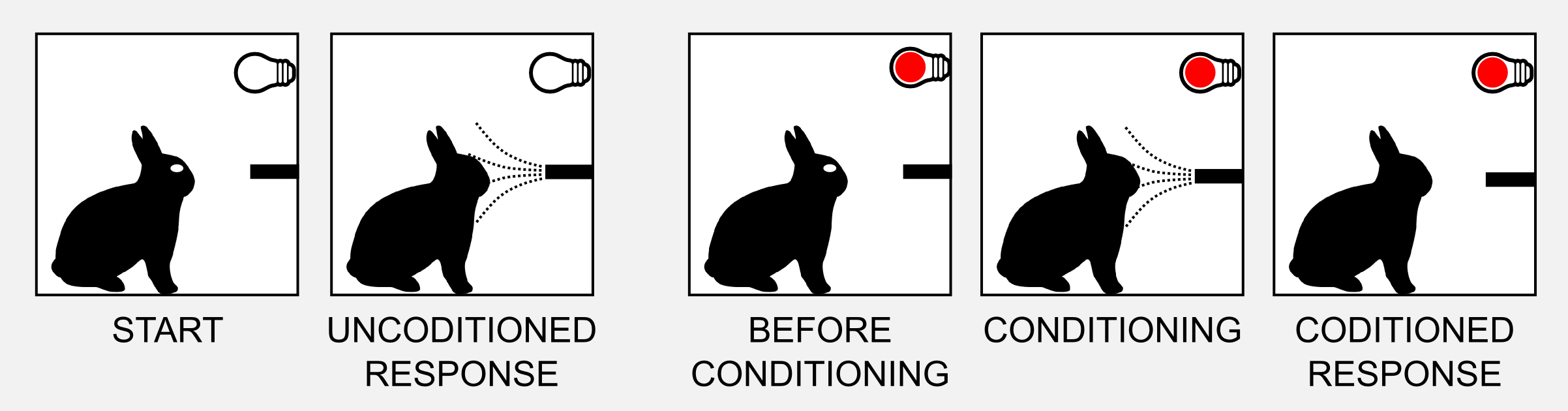
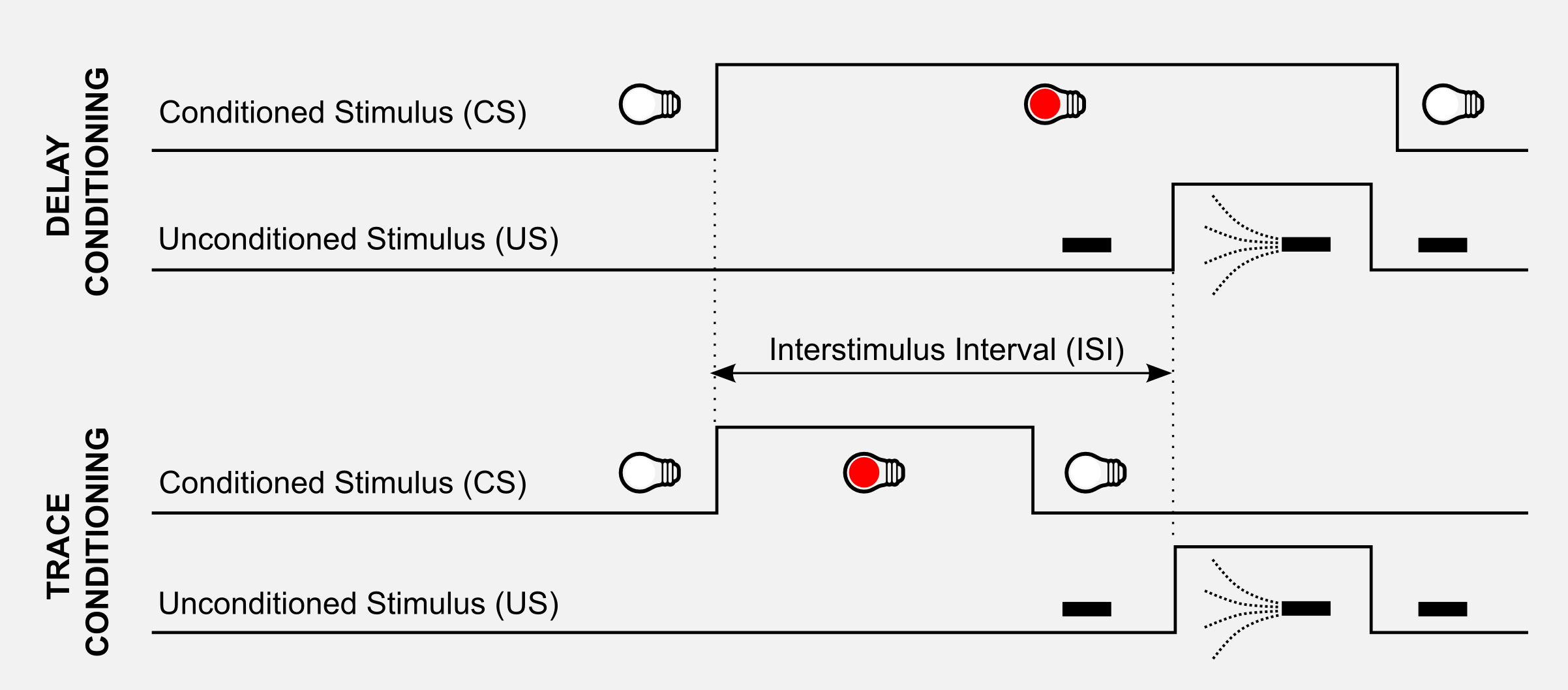
The same effect is studied with eyeblink conditioning in rabbits. A mild puff of air is directed to the rabbit’s eyes. The UR in this case is closing the eyelid, whereas the US is the air puff. During the conditioning a red light (CS) is turned on before the air puff. The conditioning creates an association between the light and the eye blinks. There are two types of arrangements of stimuli in classical conditioning experiments. In delay conditioning, the CS extends throughout the US without any interval. In trace conditioning there is a time interval, called the trace interval, between CS and US. The delay between CS and US is an important variable called interstimulus interval (ISI).
Learning about predictive relationships among stimuli is extremely important for surviving, this is the reason why it is widely present among species ranging from mice to humans. Learning means to accurately predict at each point in time the imminence-weighted sum of future US intensity levels. In the eyblinking experiment has been observed that rabbits learn a weaker prediction for CSs presented far in advance of the US. Studying the results on eyeblink conditioning, Sutton and Barto (1990) found a correlation with the TD framework. Reinforcement is weighted according to its imminence (length of the ISI), when slightly delayed it carries slightly less weight, when long-delayed it carries very little weight, and so on so forth. This assumption is the core of the TD model of classical conditioning and it is an extension of the Rescorla-Wagner model (1972). If you read the previous posts you should find some similarities whit the concept of discounted rewards. The general rule behind TD applies to rabbits and to artificial agents. This general rule can be summarised as follow:
\[\text{NewEstimate} \leftarrow \text{OldEstimate} + \text{StepSize} \big[ \text{Target} - \text{OldEstimate} \big]\]The expression \(\big[ \text{Target} - \text{OldEstimate} \big]\) is the estimation error or \(\delta\) which can be reduced moving one step towards the real value (\(\text{Target}\)). The \(\text{StepSize}\) (sometimes called learning rate) is a parameter that determines to what extent the error has to be integrated in the new estimation. If \(\text{StepSize} = 0\) the agent does not learn at all. If \(\text{StepSize} = 1\) the agent considers only the most recent information. In some application the \(\text{StepSize}\) changes at each time step. Processing the \(k\)th reward the parameter is updated as \(\frac{1}{k}\). However in practice it is often used a constant value such as 0.1 for all steps. What is the \(Target\) in our case? From the second post we know that we can estimate the utility of a state as the expectation of the returns for that state. The \(Target\) is the expected return of the state:
\[\text{Target} = E_{\pi} \Bigg[ \sum_{k=0}^{\infty} \gamma^{k} r_{t+k+1} \Bigg]\]In MC method to estimate the Target we take into account all the states visited until the end of the episode:
\[\text{Target} = E_{\pi} \Bigg[ r_{t+1} + \gamma r_{t+2} + \gamma^{2} r_{t+3} + ... + \gamma^{k} r_{t+k+1}\Bigg]\]In TD learning we want to update the utility function after each visit, therefore we do not have all the states and we do not have the values of the rewards. The only information available is \(r_{t+1}\) the reward at t+1 and the utilities estimated before. If we find a way to express the target using only those values we are done. To solve the issue we can bootstrap meaning we can use the estimates to build new estimates. This is the most important part, if we group \(\gamma\) we obtain exactly the equation of \(U(s_{t+1})\):
\[\text{Target} = E_{\pi} \Bigg[ r_{t+1} + \gamma \big( r_{t+2} + \gamma r_{t+3} + ... + \gamma^{k-1} r_{t+k+1} \big) \Bigg] = E_{\pi} \Bigg[ r_{t+1} + \gamma U(s_{t+1}) \Bigg]\]We got what we wanted. The \(\text{Target}\) is now expressed by two quantities: \(r_{t+1}\) and \(U(s_{t+1})\) and both of them are known. Taking into account all these considerations we can finally write the complete update rule:
\[U(s_{t}) \leftarrow U(s_{t}) + \alpha \big[ \text{r}_{t+1} + \gamma U(s_{t+1}) - U(s_{t}) \big]\]This update rule is fascinating. At the very first iteration we are updating the utility table using completely wrong values. Think about that, we initialized the utilities with random values (or zeros) and we are taking one of these values at \(t+1\) to update the state at \(t\). How can the algorithm converge to the real values? The magic happens when the agent meet a terminal state for the first time. In this particular case the return obtained by TD and MC coincides. Using again our cleaning robot example we can easily see what is the difference between TD and MC learning and what each one does at each step…
TD(0) Python implementation
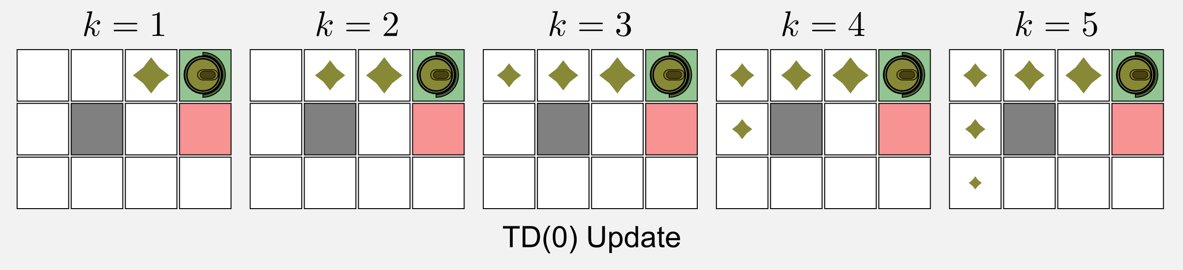
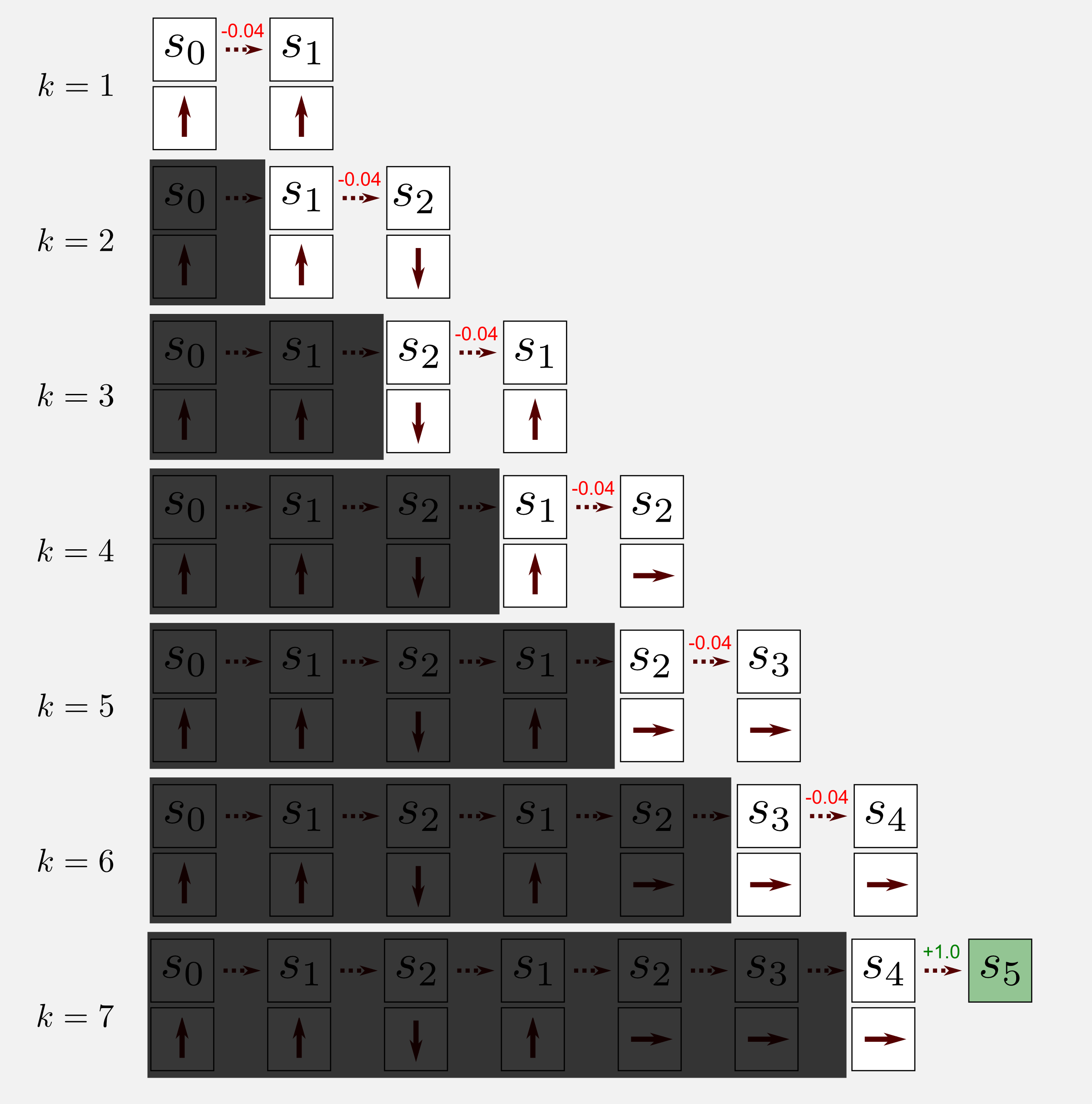
The update rule found in the previous part is the simplest form of TD learning, the TD(0) algorithm. TD(0) allows estimating the utility values following a specific policy. We are in the passive learning case for prediction, and we are in model-free reinforcement learning, meaning that we do not have the transition model. To estimate the utility function we can only move in the world. Using again the cleaning robot example I want to show you what does it mean to apply the TD algorithm to a single episode. I am going to use the episode of the second post where the robot starts at (1,1) and reaches the terminal state at (4,3) after seven steps.
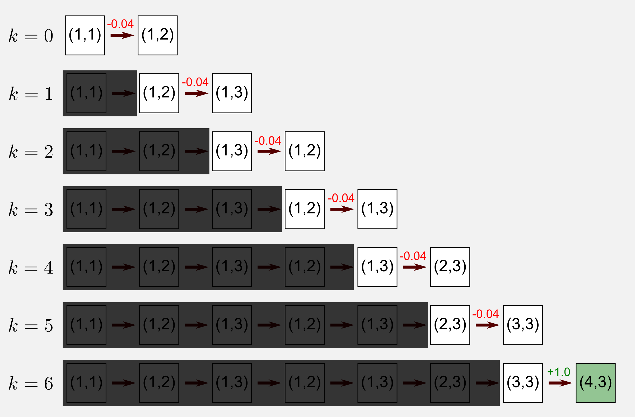
Applying the TD algorithm means to move step by step considering only the state at t and the state at t+1. That’s it, after each step we get the utility value and the reward at t+1 and we update the value at t. The TD(0) algorithm ignores the past states as shown by the shadow I added above those states. Applying the algorithm to the episode (\(\gamma = 0.9\), \(\alpha = 0.1\)) leads to the following changes in the utility matrix:
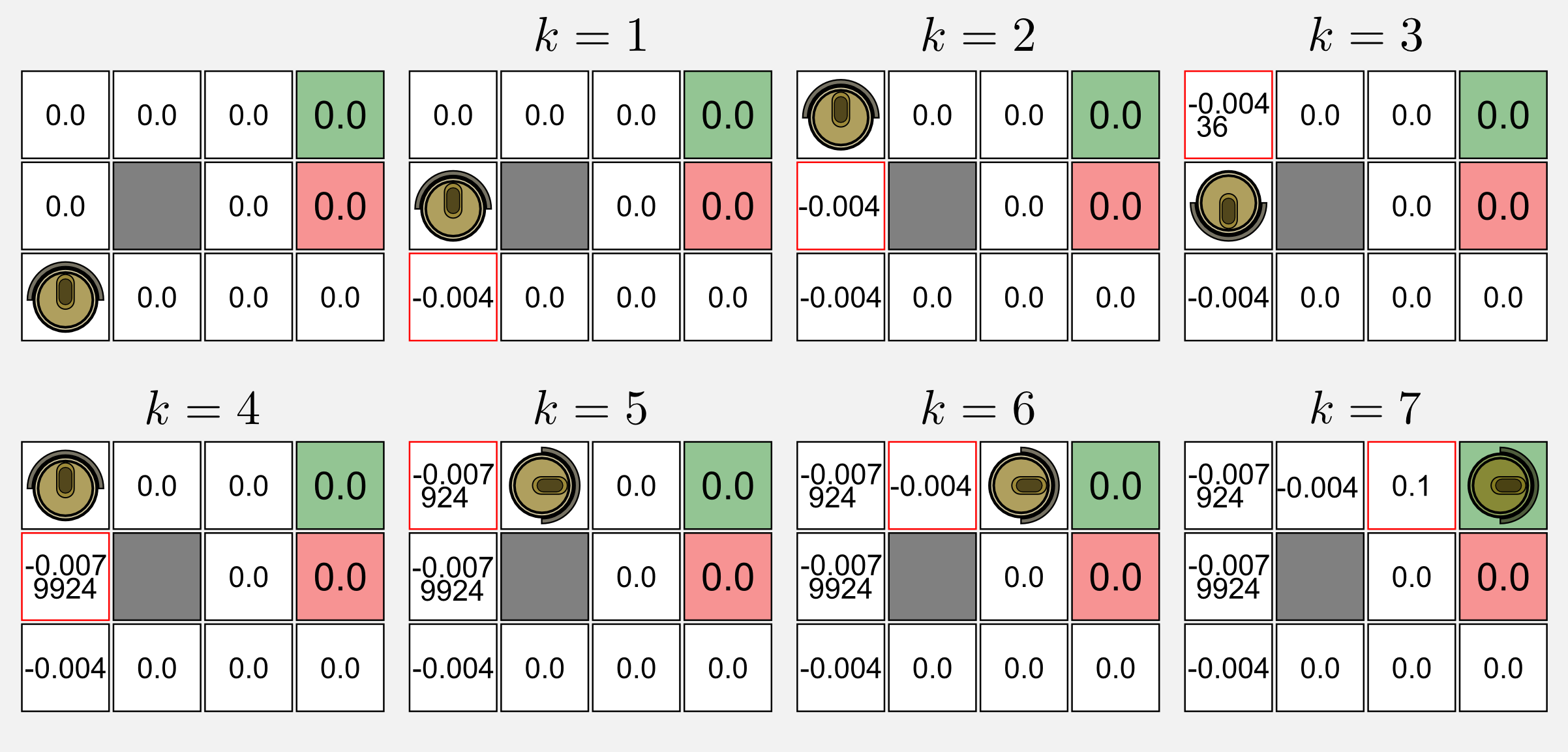
The red frame highlights the utility value that has been updated at each visit. The matrix is initialised with zeros. At k=1 the state (1,1) is updated since the robot is in the state (1,2) and the first reward (-0.04) is available. The calculation for updating the utility at (1,1) is: 0.0 + 0.1 (-0.04 + 0.9 (0.0) - 0.0) = -0.004. Similarly to (1,1) the algorithm updates the state at (1,2). At k=3 the robot goes back and the calculation take the form: 0.0 + 0.1 (-0.04 + 0.9 (-0.004) - 0.0) = -0.00436. At k=4 the robot changes again its direction. In this case the algorithm update for the second time the state (1,2) as follow: -0.004 + 0.1 (-0.04 + 0.9 (-0.00436) + 0.004) = -0.0079924. The same process is applied until the end of the episode.
In the Python implementation we have to create a grid world as we did in the second post, using the class GridWorld contained in the module gridworld.py. I will use again the 4x3 world with a charging station at (4,3) and the stairs at (4,2). The optimal policy and the utility values of this world are the same we obtained in the previous posts:
Optimal policy:			Utility Matrix:

 >   >   >   * 			0.812  0.868  0.918  1.0
 ^   #   ^   * 			0.762  0.0    0.660 -1.0
 ^   <   <   <. 		0.705  0.655  0.611  0.388
The update rule of TD(0) can be implemented in a few lines:
def update_utility(utility_matrix, observation, new_observation,
                   reward, alpha, gamma):
    '''Return the updated utility matrix

    @param utility_matrix the matrix before the update
    @param observation the state observed at t
    @param new_observation the state observed at t+1
    @param reward the reward observed after the action
    @param alpha the step size (learning rate)
    @param gamma the discount factor
    @return the updated utility matrix
    '''
    u = utility_matrix[observation[0], observation[1]]
    u_t1 = utility_matrix[new_observation[0], new_observation[1]]
    utility_matrix[observation[0], observation[1]] += \
        alpha * (reward + gamma * u_t1 - u)
    return utility_matrix
The main loop is much simpler than the one used in MC methods. In this case we do not have any first-visit constraint and the only thing to do is to apply the update rule.
for epoch in range(tot_epoch):
    #Reset and return the first observation
    observation = env.reset(exploring_starts=True)
    for step in range(1000):
        #Take the action from the action matrix
        action = policy_matrix[observation[0], observation[1]]
        #Move one step in the environment and get obs and reward
        new_observation, reward, done = env.step(action)
        #Update the utility matrix using the TD(0) rule
        utility_matrix = update_utility(utility_matrix,
                                        observation, new_observation,
                                        reward, alpha, gamma)
        observation = new_observation
        if done: break #return
The complete code, called temporal_differencing_prediction.py, is available in the GitHub repository. For the moment it is important to get the general idea behind the algorithm. Running the complete code with gamma=0.999, alpha=0.1 and following the optimal policy for a reward of -0.04 we obtain:
Utility matrix after 1 iterations:
[[-0.004  -0.0076  0.1     0.    ]
 [ 0.      0.      0.      0.    ]
 [ 0.      0.      0.      0.    ]]

Utility matrix after 2 iterations:
[[-0.00835924 -0.00085     0.186391    0.        ]
 [-0.0043996   0.          0.          0.        ]
 [-0.004       0.          0.          0.        ]]

Utility matrix after 3 iterations:
[[-0.01520748  0.01385546  0.2677519   0.        ]
 [-0.00879473  0.          0.          0.        ]
 [-0.01163916 -0.0043996  -0.004      -0.004     ]]

...

Utility matrix after 100000 iterations:
[[ 0.83573452  0.93700432  0.94746457  0.        ]
 [ 0.77458346  0.          0.55444341  0.        ]
 [ 0.73526333  0.6791969   0.62499965  0.49556852]]

...

Utility matrix after 300000 iterations:
[[ 0.85999294  0.92663558  0.99565229  0.        ]
 [ 0.79879005  0.          0.69799246  0.        ]
 [ 0.75248148  0.69574141  0.65182993  0.34041743]]
We can now compare the utility matrix obtained with TD(0) and the one obtained with Dynamic Programming in the first post:
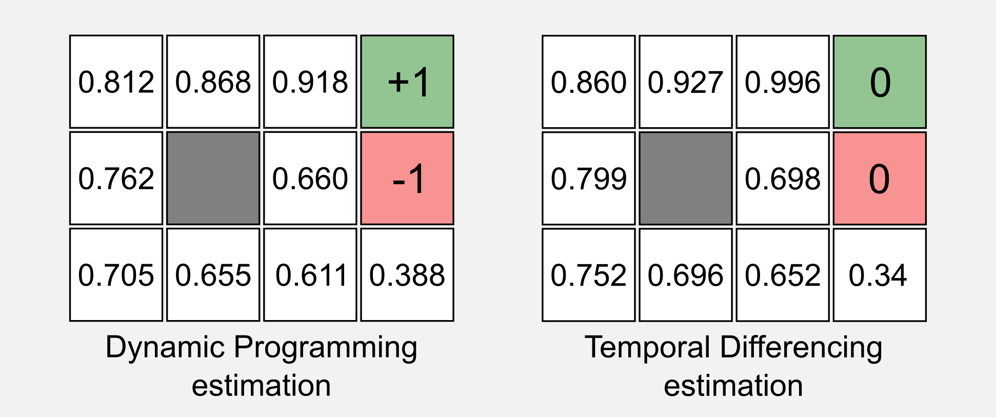
Most of the values are similar. The main difference between the two table is the estimate of the two terminal states. TD(0) does not work for terminal states because we need reward and utility of the next state at t+1. For definition after a terminal states there is no other state. However, this is not a big issue. What we want to know is the utility of the states nearby the terminal states. To overcome the problem it is often used a simple conditional statement:
if (is_terminal(state) == True):
    utility_matrix(state) = reward
Great we saw how TD(0) works, however there is something I did not talk about: what does the zero contained in the name of the algorithm means? To understand what that zero means I have to introduce the eligibility traces.
TD(λ) and eligibility traces
As I told you in the previous section, the TD(0) algorithm does not take into account past states. What matters in TD(0) is the current state and the state at t+1. However, it would be useful to extend what has been learned at t+1 also to previous states, this would accelerate the learning. To achieve this objective it is necessary to have a short-term memory mechanism to store the states that have been visited in the last steps. For each state \(s\) at time \(t\) we can define \(e_{t}(s)\) as the eligibility trace:
\[e_{t}(s) = \begin{cases} \gamma \lambda e_{t-1}(s) & \text{if}\ s \neq s_{t}; \\ \gamma \lambda e_{t-1}(s)+1 & \text{if}\ s=s_{t}; \end{cases}\]Here \(\gamma\) is the discount rate and \(\lambda \in [0,1]\) is a decay parameter called trace-decay or accumulating trace defining the update weight for each state visited. When \(0 <\lambda <\ 1\) the traces decrease in time, giving a small weight to infrequent states. For the particular case \(\lambda = 0\) we have TD(0), and only the previous prediction is updated. For \(\lambda = 1\) we have TD(1) where all the previous predictions are equally updated. TD(1) can be considered an extension of MC methods using a TD framework. In MC methods we need to wait the end of the episode in order to update the states. In TD(1) we can update all the previous states online, we do not need the end of the episode. Let’s see now what happens to a specific state trace during an episode. I will take into account an episode with seven visits where five states are visited. The state \(s_1\) is visited twice during the episode. Let’s see what happens to its trace.
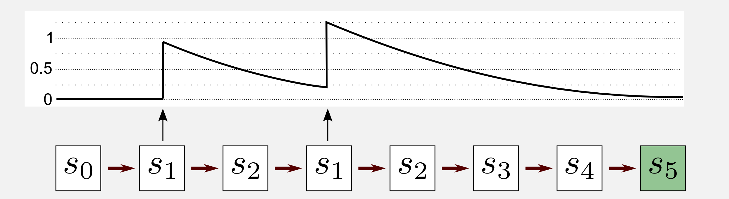
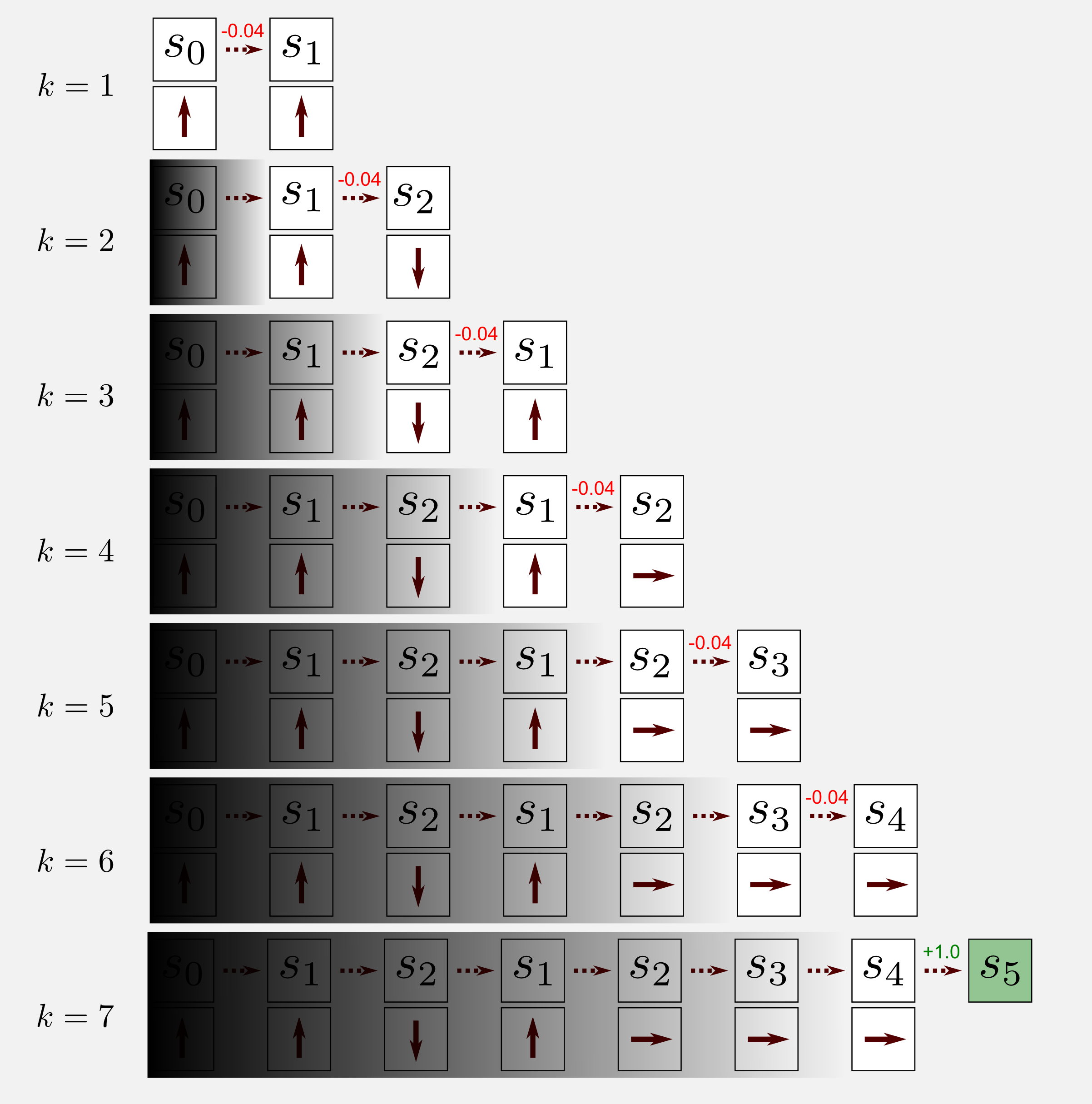
At the beginning the trace is equal to zero. After the first visit to \(s_1\) (second step) the trace goes up to 1 and then it starts decaying. After the second visit (fourth step) +1 is added to the current value (0.25) obtaining a final trace of 1.25. After that point the state \(s_1\) is no more visited and the trace slowly goes to zero. How does TD(λ) update the utility function? In TD(0) we saw that a uniform shadow was added in the graphical illustration to represent the inaccessibility of previous states. In TD(λ) the previous states are accessible but they are updated based on the eligibility trace value. States with a small eligibility trace will be updated of a small amount whereas states with high eligibility traces will be substantially updated.
Graphically we can represent TD(λ) with a non-uniform shadow partially hiding previous states. Now it’s time to define the update rule for TD(λ). Recall that the estimation error \(\delta\) was defined in the previous section as:
\[\delta_{t} = r_{t+1} + \gamma U(s_{t+1}) - U(s_{t})\]we can update the utility function as follows:
\[U_{t}(s) = U_{t}(s) + \alpha \delta_{t} e_{t}(s) \qquad \text{for all } s \in S\]To help you understand the differences between TD(0) and TD(λ) I build a 4x3 grid world where the reward is zero for all the states but the two terminal states. The utility matrix is initialised with zeros. The episode I will take into account has five visits, the robot starts at state (1,1) and it arrives at the charging station (4,3) following the optimal path.
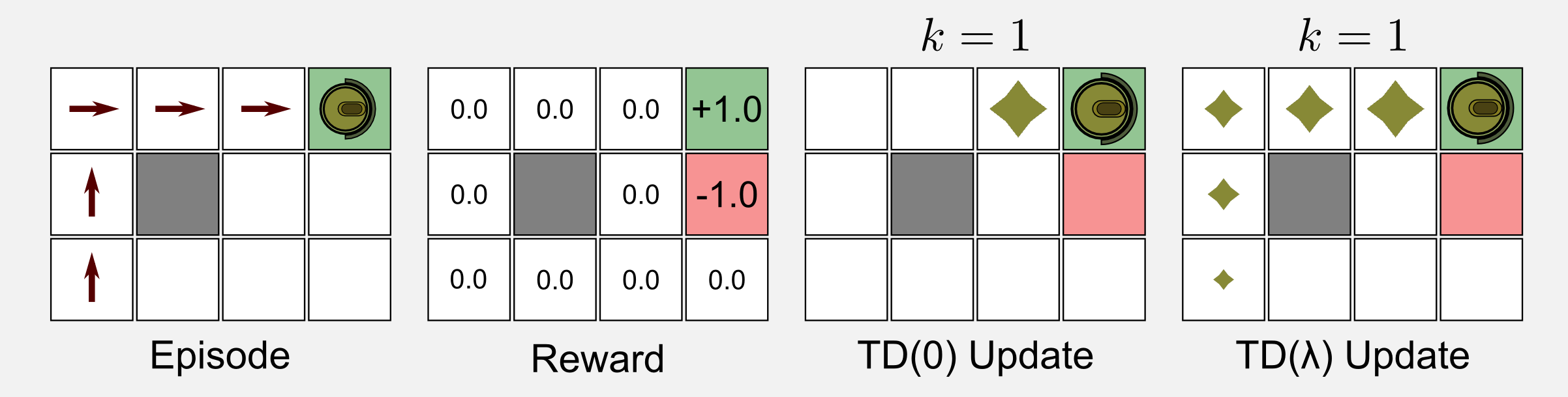
The results of the update for TD(0) and TD(λ) are the same (zero) along all the visit but the last one. When the robot reaches the charging station (reward +1.0) the update rule returns a positive value. In TD(0) the result is propagated only to the previous state (3,3). In TD(λ) the result is propagated back to all previous states thanks to the eligibility trace. The decay value of the trace gives more weight to the last states. As I told you the utility trace mechanism helps to speed up the convergence. It is easy to understand why, if you consider that in our example TD(0) needs five episodes in order to reach the same results of TD(λ).
The Python implementation of TD(λ) is straightforward. We only need to add an eligibility matrix and its update rule.
def update_utility(utility_matrix, trace_matrix, alpha, delta):
    '''Return the updated utility matrix

    @param utility_matrix the matrix before the update
    @param alpha the step size (learning rate)
    @param delta the error (Taget-OldEstimte)
    @return the updated utility matrix
    '''
    utility_matrix += alpha * delta * trace_matrix
    return utility_matrix

def update_eligibility(trace_matrix, gamma, lambda_):
    '''Return the updated trace_matrix

    @param trace_matrix the eligibility traces matrix
    @param gamma discount factor
    @param lambda_ the decaying value
    @return the updated trace_matrix
    '''
    trace_matrix = trace_matrix * gamma * lambda_
    return trace_matrix
The main loop introduces some new components compared to the TD(0) case. We have the estimation of delta in a separate line and the management of the trace_matrix in two lines. First of all the states are increased (+1) and then they are decayed.
for epoch in range(tot_epoch):
  #Reset and return the first observation
  observation = env.reset(exploring_starts=True)
  for step in range(1000):
    #Take the action from the action matrix
    action = policy_matrix[observation[0], observation[1]]
    #Move one step in the environment and get obs and reward
    new_observation, reward, done = env.step(action)
    #Estimate the error delta (Target - OldEstimate)
    delta = reward + gamma * \
        utility_matrix[new_observation[0], new_observation[1]] - \
        utility_matrix[observation[0], observation[1]]
    #Adding +1 in the trace matrix (only the state visited)
    trace_matrix[observation[0], observation[1]] += 1
    #Update the utility matrix (all the states)
    utility_matrix = update_utility(utility_matrix, trace_matrix, alpha, delta)
    #Update the trace matrix (decaying) (all the states)
    trace_matrix = update_eligibility(trace_matrix, gamma, lambda_)
    observation = new_observation
    if done: break #return
The complete code is available on the GitHub repository and it is called temporal_differencing_prediction_trace.py. Running the script we obtain the following utility matrices:
Utility matrix after 1 iterations:
[[ 0.       0.04595  0.1      0.     ]
 [ 0.       0.       0.       0.     ]
 [ 0.       0.       0.       0.     ]]

...

Utility matrix after 101 iterations:
[[ 0.90680695  0.98373981  1.05569002  0.        ]
 [ 0.8483302   0.          0.6750451   0.        ]
 [ 0.77096419  0.66967837  0.50653039  0.22760573]]

...

Utility matrix after 100001 iterations:
[[ 0.86030512  0.91323552  0.96350672  0.        ]
 [ 0.80914277  0.          0.82155788  0.        ]
 [ 0.76195244  0.71064599  0.68342933  0.48991829]]

...

Utility matrix after 300000 iterations:
[[ 0.87075806  0.92693723  0.97192601  0.        ]
 [ 0.82203398  0.          0.87812674  0.        ]
 [ 0.76923169  0.71845851  0.7037472   0.52270127]]
Comparing the final utility matrix with the one obtained without the use of eligibility traces in TD(0) you will notice similar values. One could ask: what’s the advantage of using eligibility traces? The eligibility traces version converges faster. This advantage become clear when dealing with sparse reward in a large state space. In this case the eligibility trace mechanism can considerably speeds up the convergence propagating what learnt at t+1 back to the last states visited.
SARSA: Temporal Differencing control
Now it is time to extend the TD method to the control case. Here we are in the active scenario, we want to estimate the optimal policy starting from a random one. We saw in the introduction that the final update rule for the TD(0) case was:
\[U(s_{t}) \leftarrow U(s_{t}) + \alpha \big[ \text{r}_{t+1} + \gamma U(s_{t+1}) - U(s_{t}) \big]\]The update rule is based on the tuple State-Reward-State. We are in the control case and we use the Q-function (see second post) to estimate the best policy. The Q-function requires as input a state-action pair. The TD algorithm for control is straightforward, give a look at the update rule:
\[Q(s_{t}, a_{t}) \leftarrow Q(s_{t}, a_{t}) + \alpha \big[ \text{r}_{t+1} + \gamma Q(s_{t+1}, a_{t+1}) - Q(s_{t}, a_{t}) \big]\]That’s it, we simply replaced \(U\) with \(Q\) but we must be careful because there is a difference. Now we need a new value which is the action at t+1. This is not a problem because it is contained in the Q-matrix. In TD control the estimation is based on the tuple State-Action-Reward-State-Action and this tuple gives the name to the algorithm: SARSA. SARSA has been introduced in 1994 by Rummery and Niranjan in the article “On-Line Q-Learning Using Connectionist Systems” and was originally called modified Q-learning. In 1996 Sutton introduced the current name.
To get the intuition behind the algorithm we consider again a single episode of an agent moving in a world. The robot starts at \(s_{0}\) and after seven visits it reaches a terminal state at \(s_{5}\). For each state we have an associated action. Moving forward the algorithm takes into account only the state at t and t+1. In the standard implementation of SARSA the previous states are ignored, as shown by the shadow on top of them in the graphical illustration. This is in line with the TD framework as explained in the TD(0) section. Now I would like to summarise all the steps of the algorithm:
- Move one step selecting \(a_{t}\) from \(\pi(s_{t})\)
- Observe: \(r_{t+1}\), \(s_{t+1}\), \(a_{t+1}\)
- Update the state-action function \(Q(s_{t}, a_{t})\)
- Update the policy \(\pi(s_{t}) \leftarrow \underset{a}{\text{ argmax }} Q(s_{t},a_{t})\)
In step 1 the agent selects one action from the policy and moves one step forward. In step 2 the agent observes the reward, the new state and the associated action. In step 3 the algorithm updates the state-action function using the update rule. In step 4 we are using the same mechanism of MC for control (see second post), the policy \(\pi\) is updated at each visit choosing the action with the highest state-action value. We are making the policy greedy. As for MC methods we use the exploring starts condition.
Can we apply the TD(λ) ideas to SARSA? Yes we can. SARSA(λ) follows the same steps of TD(λ) implementing the eligibility traces to speed up the convergence. The intuition behind the algorithm is the same but instead of applying the prediction method to the states, SARSA(λ) applies it to state-action pairs. We have a trace for each state-action and this trace is updated as follows:
\[e_{t}(s,a) = \begin{cases} \gamma \lambda e_{t-1}(s,a)+1 & \text{if}\ s=s_{t} \text{ and } a=a_{t}; \\ \gamma \lambda e_{t-1}(s,a) & \text{otherwise}; \end{cases}\]To update the Q-function we use the following update rule:
\[Q_{t+1}(s, a) = Q_{t}(s, a) + \alpha \delta_{t} e_{t}(s, a) \qquad \text{for all } s \in S\]Considering that in this post I introduced many new concepts I will not proceed with the Python implementation of SARSA(λ). Consider it an homework and try to implement it by yourself. If what explained in the previous sections is not enough you can read the chapter 7.5 of Sutton and Barto’s book.
SARSA: Python and ε-greedy policy
The Python implementation of SARSA requires a Numpy matrix called state_action_matrix which can be initialised with random values or filled with zeros. Here you must remember that we defined state_action_matrix has having one state for each column, and one action for each row (see second post). For instance in the 4x3 grid world, with the query state_action_matrix[0, 2] we get the state-action value for the state (1,3) (top-left corner) and action DOWN. With the query state_action_matrix[11, 0] we get the state-action value for the state (4,1) (bottom-right corner) and action UP. This follows the convention of Russel and Norvig for naming the states with the bottom-left corner being the state (1,1). Note that in Python we use the Numpy convention where [0, 0] defines the top-left value of the grid world. SARSA is based on the following update rule for the state-action matrix:
def update_state_action(state_action_matrix, observation, new_observation,
                   action, new_action, reward, alpha, gamma):
    '''Return the updated utility matrix

    @param state_action_matrix the matrix before the update
    @param observation the state observed at t
    @param new_observation the state observed at t+1
    @param action the action at t
    @param new_action the action at t+1
    @param reward the reward observed after the action
    @param alpha the step size (learning rate)
    @param gamma the discount factor
    @return the updated state action matrix
    '''
    #Getting the values of Q at t and at t+1
    col = observation[1] + (observation[0]*4)
    q = state_action_matrix[action ,col]
    col_t1 = new_observation[1] + (new_observation[0]*4)
    q_t1 = state_action_matrix[new_action ,col_t1]
    #Applying the update rule
    state_action_matrix[action ,col] += \
        alpha * (reward + gamma * q_t1 - q)
    return state_action_matrix
Moreover, since we are in the control case and we want to estimate a policy, we need also an update function to achieve this goal:
def update_policy(policy_matrix, state_action_matrix, observation):
    '''Return the updated policy matrix

    @param policy_matrix the matrix before the update
    @param state_action_matrix the state-action matrix
    @param observation the state obsrved at t
    @return the updated state action matrix
    '''
    col = observation[1] + (observation[0]*4)
    #Getting the index of the action with the highest utility
    best_action = np.argmax(state_action_matrix[:, col])
    #Updating the policy
    policy_matrix[observation[0], observation[1]] = best_action
    return policy_matrix
The update_policy function makes the policy greedy selecting the action with the highest value in accordance with the step 4 of the algorithm. Finally, the main loop updates the state_action_matrix and the policy_matrix for each visit in the episode.
for epoch in range(tot_epoch):
  #Reset and return the first observation
  observation = env.reset(exploring_starts=True)
  for step in range(1000):
    #Take the action from the action matrix
    action = policy_matrix[observation[0], observation[1]]
    #Move one step in the environment and get obs,reward and new action
    new_observation, reward, done = env.step(action)
    new_action = policy_matrix[new_observation[0], new_observation[1]]
    #Updating the state-action matrix
    state_action_matrix = update_state_action(state_action_matrix,
                                              observation, new_observation,
                                              action, new_action,
                                              reward, alpha, gamma)
    #Updating the policy
    policy_matrix = update_policy(policy_matrix,
                                  state_action_matrix,
                                  observation)
    observation = new_observation
    if done: break
The complete Python script is available in the GitHub repository and is called temporal_differencing_control_sarsa.py.
Running the script with alpha=0.001 and gamma=0.999 gives the optimal policy after 180000 iterations.
Policy matrix after 1 iterations:
 <   v   >   *
 ^   #   v   *
 >   v   v   >

...

Policy matrix after 90001 iterations:
 >   >   >   *
 ^   #   ^   *
 ^   <   ^   <

...

Policy matrix after 180001 iterations:
 >   >   >   *
 ^   #   ^   *
 ^   <   <   <
Does SARSA always converge to the optimal policy? The answer is yes, SARSA converges with probability 1 as long as all the state-action pairs are visited an infinite number of times. This assumption is called by Russel and Norvig Greedy in the Limit of Infinite Exploration (GLIE). A GLIE scheme must try each action in each state an unbounded number of times to avoid having a finite probability that an optimal action is missed because of an unusually bad series of outcomes. In our grid world it can happen that an unlucky initialization causes a bad policy that keeps the agent far from certain states. In the second post we used the assumption of exploring starts to guarantee a uniform exploration of all the state-action pairs. However, exploring starts can be hard to apply in a large state space. An alternative solution is called ε-greedy policy. An ε-greedy policy explores all the states taking the action with the highest value but with a small probability ε it selects an action at random. After defining \(0 \leq \sigma \leq 1\) as a uniform random number drawn at each time step, and \(A\) as the set containing all the available action, we select the action \(a\) as follow:
\[\pi(s) = \begin{cases} \underset{a}{\text{ argmax }} Q(s, a) & \text{if}\ \sigma > \epsilon; \\ a \sim A(s) & \text{if}\ \sigma \leq \epsilon; \end{cases}\]In Python we can easily implement a function that returns an action following the ε-greedy scheme:
def return_epsilon_greedy_action(policy_matrix, observation, epsilon=0.1):
    tot_actions = int(np.nanmax(policy_matrix) + 1)
    #Getting the greedy action
    action = int(policy_matrix[observation[0], observation[1]])
    #Probabilities of non-greedy actions
    non_greedy_prob = epsilon / tot_actions
    #Probability of the greedy action
    greedy_prob = 1 - epsilon + non_greedy_prob
    #Array containing a weight for each action
    weight_array = np.full((tot_actions), non_greedy_prob)
    weight_array[action] = greedy_prob
    #Sampling the action based on the weights
    return np.random.choice(tot_actions, 1, p=weight_array)
In the naive implementation of ε-greedy policy at each non-greedy action is given the same probability, but some actions may be better than others. Using a softmax distribution (e.g. Boltzmann distribution) it is possible to give the highest probability to the greedy action without treating the others in the same way. Here, for simplicity I will use the naive approach.
The exploring starts and ε-greedy policy do not exclude one another, they can coexist. Using the two approaches at the same time can give to faster convergence. Let’s try to extend the previous script with ε-greedy action selection to see what happens.
In the main loop we have to replace the standard action selection with the ε-greedy action. Running the script with gamma=0.999, alpha=0.001 and epsilon=0.1 gives the optimal policy in 130000 iterations, meaning 50000 iterations less. The complete code is part of the file temporal_differencing_control_sarsa.py you can enable or disable the ε-greedy selection commenting the corresponding line in the main loop.
How to choose the value of ε? Most of the time a value of 0.1 is a good choice. Choosing a value that is too high will cause the algorithm to converge slowly (too much exploration). On the other hand, a value which is too small does not guarantee to visit all the state-action pairs leading to sub-optimal policies. This issue is known as the exploration-exploitation dilemma and is one of the problems afflicting reinforcement learning. It is time to introduce Q-learning, another algorithm for TD control estimation.
Q-learning: off-policy control
Q-learning was introduced by Watkins in his doctoral dissertation and is considered one of the most important algorithm in reinforcement learning. Understanding how it works means understanding most of the following posts. Before proceeding any further, make sure you got the following key concepts:
- The Generalised Policy Iteration (GPI) (second post)
- The \(\text{Target}\) term in TD learning (first section)
- The update rule of SARSA (previous section)
Now we can proceed. In the control case we always used the policy \(\pi\) to learn on the run, meaning that we updated \(\pi\) from experiences sampled from \(\pi\). This approach is called on-policy learning. There is another way to learn about \(\pi\) which is called off-policy learning. In off-policy learning we do not need a policy in order to update our Q-function. Of course we can still generate a policy \(\pi\) based on the action with the maximum utility (taken from our Q-function) but the Q-function itself is updated thanks to a second policy \(\mu\) that is not updated. For instance, consider the first four iterations of an off-policy algorithm applied to the 4x3 grid world. We can see how after the random initialisation of \(\pi\) the states are updated step by step, whereas the policy \(\mu\) does not change at all.
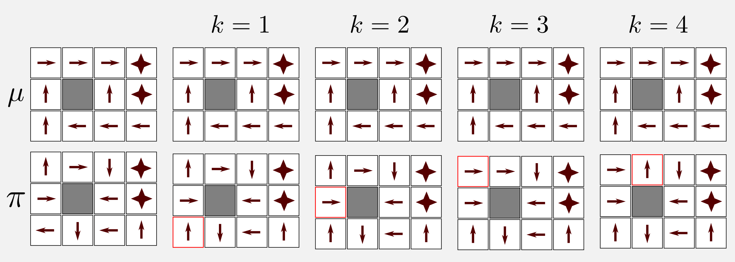
What are the advantages of off-policy learning? First of all using off-policy it is possible to learn about an optimal policy while following an exploratory policy \(\mu\). Off-policy means learning by observation. For example, we can find an optimal policy looking to a robot that is following a sub-optimal policy. It is also possible to learn about multiple policies while following one policy (e.g. multi-robot scenario). Moreover, in deep reinforcement learning we will see how off-policy allows re-using old experiences generated from old policies to improve the current policy (experience replay). The most famous off-policy TD algorithm for control is called Q-Learning. To understand how Q-learning works let’s consider its update rule:
\[Q(s_{t}, a_{t}) \leftarrow Q(s_{t}, a_{t}) + \alpha \big[ \text{r}_{t+1} + \gamma \underset{a}{\text{ max }} Q(s_{t+1}, a) - Q(s_{t}, a_{t}) \big]\]Comparing the update rule of SARSA and the one of Q-learning you will notice only one difference: the \(\text{Target}\) term. Here I report both of them to simplify the comparison:
\[\text{Target}[\text{SARSA}] = \text{r}_{t+1} + \gamma Q(s_{t+1}, a_{t+1})\] \[\text{Target}[\text{Q-learning}] = \text{r}_{t+1} + \gamma \underset{a}{\text{ max }} Q(s_{t+1}, a)\]SARSA uses GPI to improve the policy \(\pi\). The \(\text{Target}\) is estimated through \(Q(s_{t+1}, a_{t+1})\) that is based on the action \(a_{t+1}\) sampled from the policy \(\pi\). In SARSA improving \(\pi\) means improving the estimation returned by \(Q(s_{t+1}, a_{t+1})\). In Q-learning we have two policies \(\pi\) and \(\mu\). The action value \(a\) necessary to estimate \(Q(s_{t},a)\) is directly taken from the Q-function using the \(\text{ max }\) operator. Q-learning makes an update based on the greedy Q-value of the successor state, \(s_{t+1}\), while SARSA uses the Q-value of the action \(a_{t+1}\) chosen by the learning policy. This makes SARSA an on-policy algorithm, with convergence depending on the learning policy. Q-learning does not depend on the policy and it can converge following a completely random one. Now I would like to better describe the \(\text{Target}\) term used in Q-learning. First of all, let’s recall that the value of \(a_{t+1}\) cannot be sampled from the policy \(\mu\) because it is not updated during the training (using it would break the GPI scheme). However, having the Q-function we can update at each time step the policy \(\pi\) as follows:
\[\pi(s_{t+1}) = \underset{a}{\text{ argmax }} Q(s_{t+1},a)\]At this point it is obvious that we do not really need the policy \(\pi\) for choosing the action, we can simply use the term on the right and rewrite the \(\text{Target}\) as the discounted Q-value obtained at \(s_{t+1}\) through a greedy selection:
\[\text{Target} = \text{r}_{t+1} + \gamma Q(s_{t+1}, \underset{a}{\text{ argmax }} Q(s_{t+1},a))\]The expression below corresponds to the highest Q-value at t+1 meaning that it can be reduced to:
\[\text{Target} = \text{r}_{t+1} + \gamma \underset{a}{\text{ max }} Q(s_{t+1}, a)\]That’s it, we have the \(\text{Target}\) used in the actual update rule and this value follows the GPI scheme. Let’s see now all the steps involved in Q-learning:
- Move one step selecting \(a_{t}\) from \(\mu(s_{t})\)
- Observe: \(r_{t+1}\), \(s_{t+1}\)
- Update the state-action function \(Q(s_{t}, a_{t})\)
- (optional) Update the policy \(\pi(s_{t}) \leftarrow \underset{a}{\text{ argmax }} Q(s_{t},a)\)
There are some differences between the steps followed in SARSA and the one followed in Q-learning. Unlike SARSA, step 2 of Q-learning does not consider \(a_{t+1}\), the action at the next step. In this sense Q-learning updates the state-action function using the tuple State-Action-Reward-State. Comparing step 1 and step 4 you can see that in step 1 of SARSA the action is sampled from \(\pi\) and then the same policy is updated at step 4. In step 1 and step 4 of Q-learning we are sampling the action from the exploration policy \(\mu\) and (optionally) we update the policy \(\pi\) at step 4. The step 4 is optional because the action value can be obtained directly from the Q-function, calculating and storing \(\pi\) can be a waste of resources.
Also for Q-learning there is a version based on eligibility traces. Actually there are two versions: Watkins’s Q(λ) and Peng’s Q(λ). Here, I will focus on Watkins’s Q(λ). The Q(λ) algorithm was introduced by Watkins in his doctoral dissertation. The idea behind the algorithm is similar to TD(λ) and SARSA(λ). Like in SARSA(λ) we are updating state-action pairs, with an important difference. In Q-learning there are two policies, the exploratory policy \(\mu\) used to sample actions and the target policy \(\pi\) updated at each iteration. Because the action \(a\) is chosen with ε-greedy, there is a chance to select an exploratory action instead of a greedy one. In this case the eligibility traces for all state-action pairs but the current one are set to zero.
\[e_{t}(s,a) = I_{ss_{t}} \cdot I_{aa_{t}} + \begin{cases} \gamma \lambda e_{t-1}(s,a) & \text{if}\ Q_{t-1}(s_{t},a_{t})= \underset{a}{\text{max }} Q_{t-1}(s_{t},a); \\ 0 & \text{otherwise}; \end{cases}\]The term \(I_{ss_{t}}\) is an identity indicator and it is equal to 1 if \(s=s_{t}\). The same for \(I_{aa_{t}}\). The estimation error \(\delta\) is defined as:
\[\delta_{s} = r_{t+1} + \gamma \underset{a}{\text{max }} Q_{t}(s_{t+1},a) - Q_{t}(s_{t},a_{t})\]To update the Q-function we use the following update rule:
\[Q_{t+1}(s, a) = Q_{t}(s, a) + \alpha \delta_{t} e_{t}(s, a) \qquad \text{for all } s \in S\]Unfortunately, cutting off traces when an exploratory non-greedy action is taken loses much of the advantages of using eligibility traces. Like for SARSA(λ) I will not implement the Q(λ) algorithm in the next section to keep the post more compact. However a good pseudo-code is given in chapter 7.6 of the Sutton and Barto’s book.
Q-learning: Python implementation
The Python implementation of the algorithm requires a random policy called policy_matrix and an exploratory policy called exploratory_policy_matrix. The first can be initialised randomly, whereas the second can be any sub-optimal policy. The action to be executed at each visit are taken from exploratory_policy_matrix, whereas the update rule of step 4 is applied to the policy_matrix. The code is very similar to the one used in SARSA, the main difference is in the update rule for the state-action matrix:
def update_state_action(state_action_matrix, observation, new_observation,
                        action, reward, alpha, gamma):
    '''Return the updated utility matrix

    @param state_action_matrix the matrix before the update
    @param observation the state obsrved at t
    @param new_observation the state observed at t+1
    @param action the action at t
    @param new_action the action at t+1
    @param reward the reward observed after the action
    @param alpha the ste size (learning rate)
    @param gamma the discount factor
    @return the updated state action matrix
    '''
    #Getting the values of Q at t and at t+1
    col = observation[1] + (observation[0]*4)
    q = state_action_matrix[action ,col]
    col_t1 = new_observation[1] + (new_observation[0]*4)
    q_t1 = np.max(state_action_matrix[: ,col_t1])
    #Applying the update rule
    state_action_matrix[action ,col] += alpha * (reward + gamma * q_t1 - q)
    return state_action_matrix
Time for an example. Let’s suppose you noticed that the cleaning robot bought last week does not follow an optimal policy while going back to the charging station. The robot is following a sub-optimal path that is unsafe. You want to find an optimal policy and propose an upgrade to the manufacturer (and get hired!). There is a problem, you do not have any access to the robot firmware. The robot is following its internal policy \(\mu\) and this policy is inaccessible. What to do?
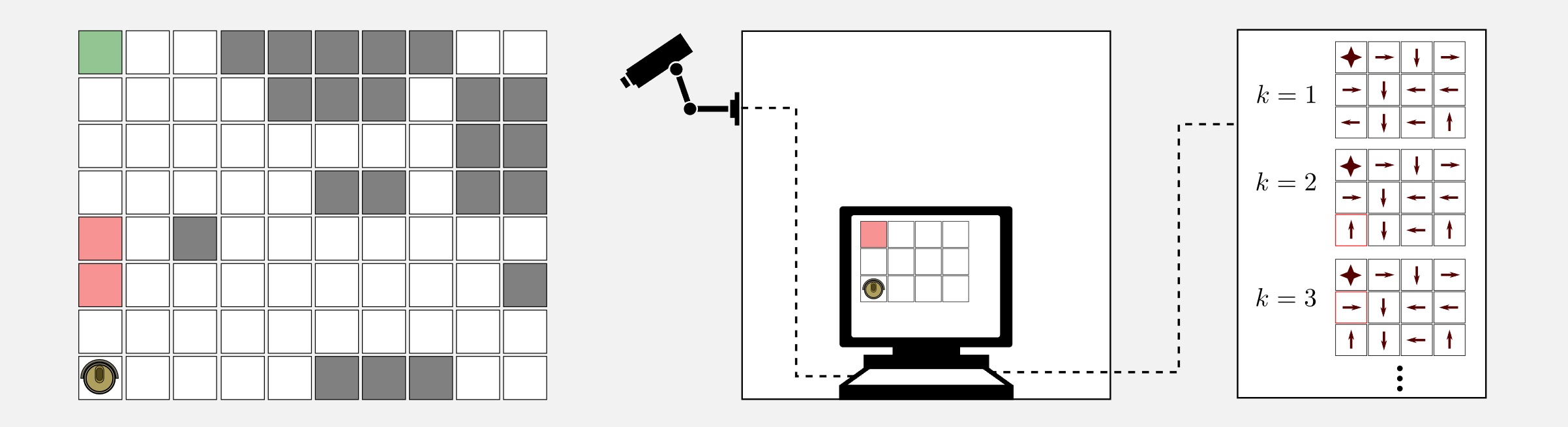
What you can do is to use an off-policy algorithm like Q-learning to estimate an optimal policy. First of all you create a discrete version of the room using the GridWorld class. Second, you get a camera and thanks to some markers you estimate the position of the robot in the real world, then relocate it in the grid world. At each time step you have the position of the robot and the reward. The camera is connected to your workstation and in the workstation is running the Q-learning Python script. Fortunately you do not have to write the code from scratch because you notice that a good starting script is available on the dissecting-reinforcement-learning official repository on GitHub and is called temporal_differencing_control_qlearning.py. The script is based on the usual 4x3 grid world, but can be easily extended to more complex scenarios.
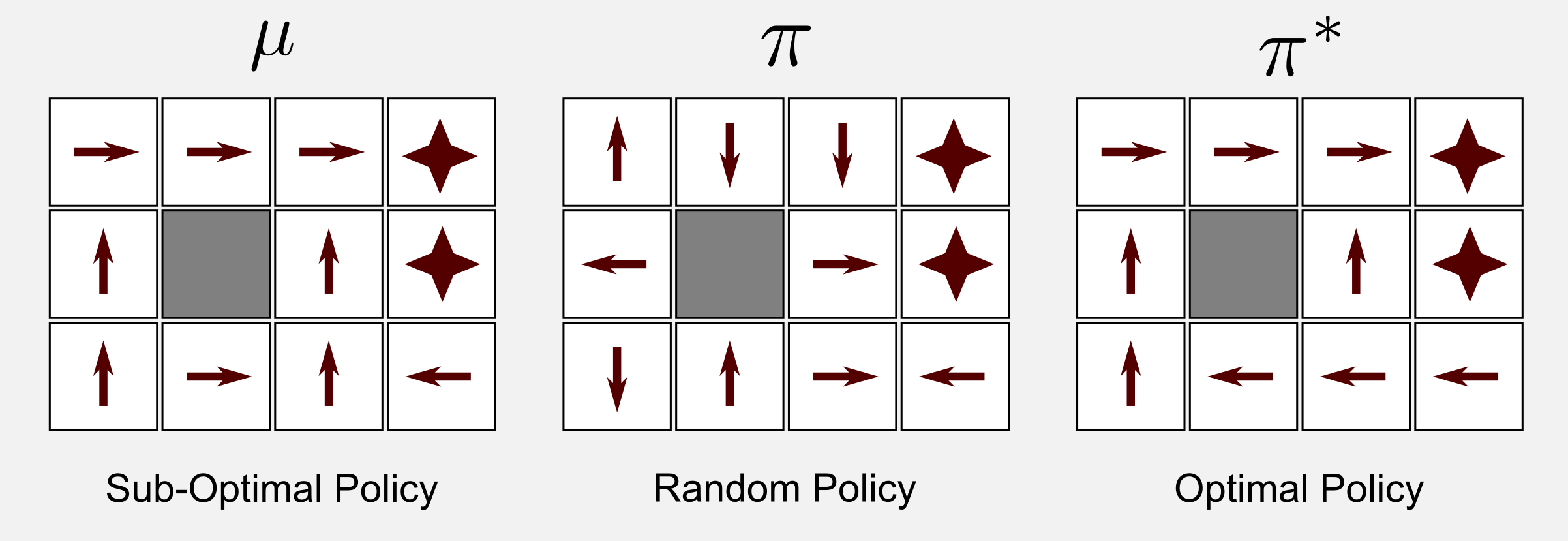
Running the script with alpha=0.001, gamma=0.999 and epsilon=0.1 the algorithm converged to the optimal policy in 300000 iterations. Great! You got the optimal policy. However there are two important limitations. First, the algorithm converged after 300000 iterations, meaning that you need 300000 episodes. Probably you have to monitor the robot for months in order to get all these episodes. In a deterministic environment you can estimate the policy \(\mu\) through observation and then run the 300000 episodes in simulation. However, in environments that are non-deterministic you need to spend much more energies in order to find the motion model. This is very time consuming. The second limitation is that the optimal policy is valid only for the current room setup. When you change the position of the charging station or the position of the obstacles you have to find a new policy. We will see in a future post how to generalise to much larger state space using supervised learning and neural networks. For the moment let’s focus on the results achieved. Q-learning followed a policy \(\mu\) which was sub-optimal and estimated the optimal policy \(\pi^{*}\) starting from a random policy \(\pi\).
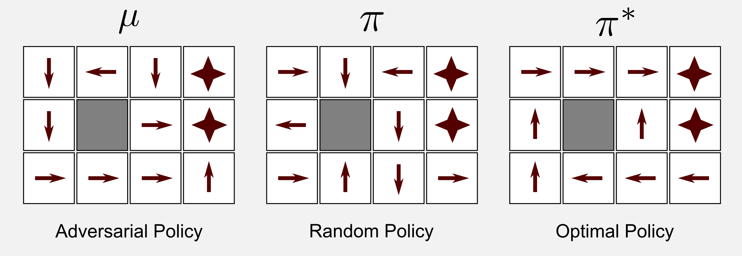
What is interesting about Q-learning is that it converges also when the policy \(\mu\) is an adversarial policy. Let’s suppose that \(\mu\) pushes the robot as far as possible from the charging station and as close as possible to the stairs. Is the algorithm going to converge in these extreme conditions? Yes. Running the script with the same parameters and with an adversarial policy the algorithm converges to the optimal policy in 583001 iterations. We empirically demonstrated that starting from a favourable policy speeds up convergence.
Conclusions
This post has summarised many important concepts in reinforcement learning. TD methods are widely used because of their simplicity and versatility. As in the second post we divided TD methods in two families: prediction and control. The prediction TD algorithm has been called TD(0). Via eligibility traces it is possible to extend to previous states what has been learnt in the last one. The extension of TD(0) with eligibility traces is called TD(λ). The control algorithms in TD are called SARSA and Q-learning. The former is an on-policy algorithm that updates the policy while moving in the environment. The latter is an off-policy algorithm based on two separate policies, one updated and the other used for moving in the world. Do TD methods converge faster than MC methods? There is no mathematical proof but by experience TD methods converge faster.
Index
- [First Post] Markov Decision Process, Bellman Equation, Value iteration and Policy Iteration algorithms.
- [Second Post] Monte Carlo Intuition, Monte Carlo methods, Prediction and Control, Generalised Policy Iteration, Q-function.
- [Third Post] Temporal Differencing intuition, Animal Learning, TD(0), TD(λ) and Eligibility Traces, SARSA, Q-learning.
- [Fourth Post] Neurobiology behind Actor-Critic methods, computational Actor-Critic methods, Actor-only and Critic-only methods.
- [Fifth Post] Evolutionary Algorithms introduction, Genetic Algorithms in Reinforcement Learning, Genetic Algorithms for policy selection.
- [Sixt Post] Reinforcement learning applications, Multi-Armed Bandit, Mountain Car, Inverted Pendulum, Drone landing, Hard problems.
- [Seventh Post] Function approximation, Intuition, Linear approximator, Applications, High-order approximators.
- [Eighth Post] Non-linear function approximation, Perceptron, Multi Layer Perceptron, Applications, Policy Gradient.
Resources
-
The complete code for TD prediction and TD control is available on the dissecting-reinforcement-learning official repository on GitHub.
-
Dadid Silver’s course (DeepMind) in particular lesson 4 [pdf][video] and lesson 5 [pdf][video]
-
Christopher Watkins doctoral dissertation, which introduced the Q-learning for the first time [pdf]
-
Machine Learning Mitchell T. (1997) [web]
-
Artificial intelligence: a modern approach. (chapters 17 and 21) Russell, S. J., Norvig, P., Canny, J. F., Malik, J. M., & Edwards, D. D. (2003). Upper Saddle River: Prentice hall. [web] [github]
-
Reinforcement learning: An introduction. Sutton, R. S., & Barto, A. G. (1998). Cambridge: MIT press. [html]
-
Reinforcement learning: An introduction (second edition). Sutton, R. S., & Barto, A. G. (2018). [pdf]
References
Bellman, R. (1957). A Markovian decision process (No. P-1066). RAND CORP SANTA MONICA CA.
Rescorla, R. A., & Wagner, A. R. (1972). A theory of Pavlovian conditioning: Variations in the effectiveness of reinforcement and nonreinforcement. Classical conditioning II: Current research and theory, 2, 64-99.
Rummery, G. A., & Niranjan, M. (1994). On-line Q-learning using connectionist systems. University of Cambridge, Department of Engineering.
Russell, S. J., Norvig, P., Canny, J. F., Malik, J. M., & Edwards, D. D. (2003). Artificial intelligence: a modern approach (Vol. 2). Upper Saddle River: Prentice hall.
Sutton, R. S. (1988). Learning to predict by the methods of temporal differences. Machine learning, 3(1), 9-44.
Sutton, R. S., & Barto, A. G. (1990). Time-derivative models of pavlovian reinforcement.
Watkins, C. J. C. H. (1989). Learning from delayed rewards (Doctoral dissertation, University of Cambridge).