Dissecting Reinforcement Learning-Part.2

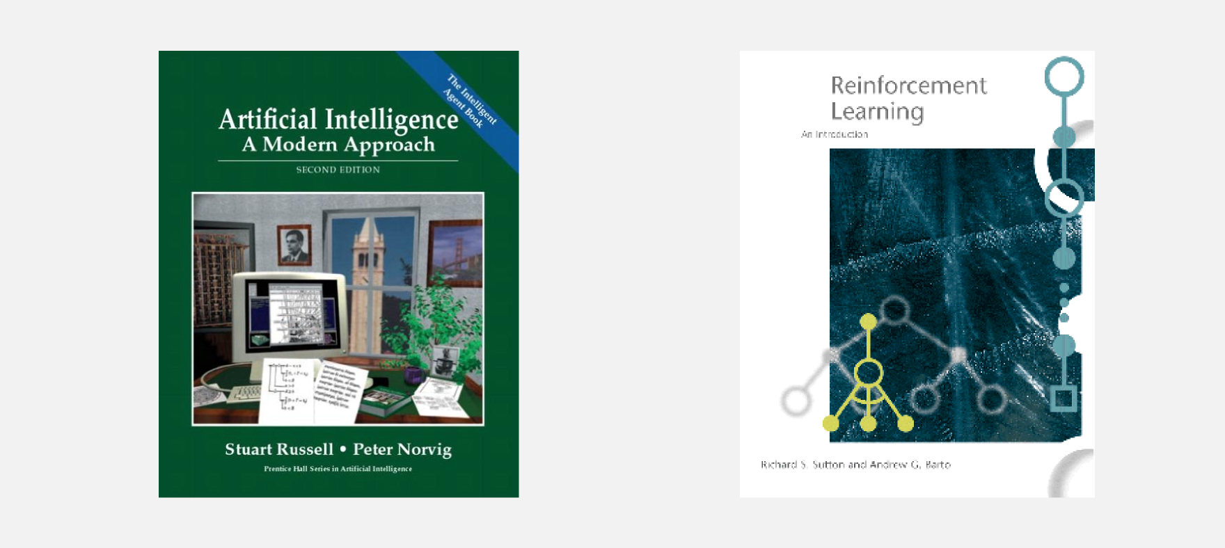
Welcome to the second part of the dissecting reinforcement learning series. If you managed to survive to the first part then congratulations! You learnt the foundation of reinforcement learning, the dynamic programming approach. As I promised in the second part I will go deeper in model-free reinforcement learning (for prediction and control), giving an overview on Monte Carlo (MC) methods. This post is (weakly) connected to part one, and I will use the same terminology, examples and mathematical notation. I will merge some of the ideas presented by Russel and Norvig in Artificial Intelligence: A Modern Approach and the classical Reinforcement Learning, An Introduction by Sutton and Barto. In particular I will focus on chapter 21 (second edition) of the former and on chapter 5 (first edition) of the latter. Moreover, you can follow lecture 4 and lecture 5 of David Silver’s course. For open versions of the books look at the resource section.

All right, now with the same spirit of the previous part I am going to dissect one-by-one all the concepts we will step through.

Beyond dynamic programming

In the first post I introduced the two main algorithms for computing optimal policies: value iteration and policy iteration. We modelled the environment as a Markov decision process (MDP), and we used a transition model to describe the probability of moving from one state to the other. The transition model was stored in a matrix T and used to find the utility function \(U^{*}\) and the best policy \(\pi^{*}\). Here, we must be careful with the mathematical notation. In the book of Sutton and Barto the utility function is called value function or state-value function and is indicated with the letter \(V\). In order to keep everything uniform I will use the notation of Russel and Norvig which uses the letter \(U\) to identify the utility function. The two notations have the same meaning and they define the value of a state as the expected cumulative future discounted reward starting from that state. The reader should get used to different notations as a good form of mental gymnastics.

Now, I would like to give a proper definition of model-free reinforcement learning and in particular of passive and active reinforcement learning. In model-free reinforcement learning the first thing we miss is a transition model. In fact the name model-free stands for transition-model-free. The second thing we miss is the reward function \(R(s)\) giving to the agent the reward associated to a particular state. In the passive approach we have a policy \(\pi\) used by the agent to move in the environment. In state \(s\) the agent always produces the action \(a\) given by the policy \(\pi\). The goal of the agent in passive reinforcement learning is to learn the utility function \(U^{\pi}(s)\). Sutton and Barto called this case MC for prediction. It is also possible to estimate the optimal policy while moving in the environment. In this case we are in an active case and using the words of Sutton and Burto we will say that we are applying MC for control estimation. Here, I will use again the example of the cleaning robot from the first post but with a different setup.

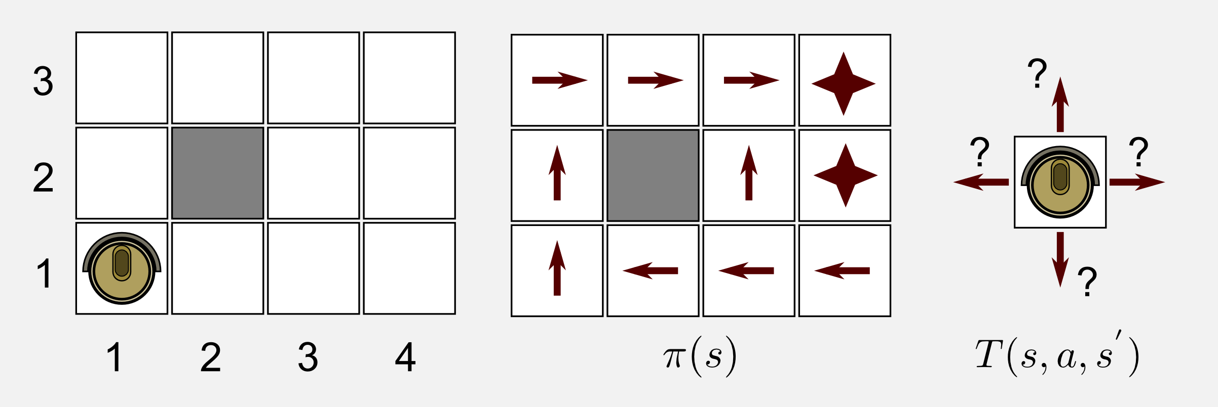
The robot is in a 4x3 world with an unknown transition model. The only information about the environment is the states availability. Since the robot does not have the reward function it does not know which state contains the charging station (+1) and which state contains the stairs (-1). Only in the passive case the robot has a policy that can follow to move in the world. Finally, the transition model, since the robot does not know what it is going to happen after each action it can only give unknown probabilities to each possible outcome. To summarize, in the passive case this is what we have:

1. Set of possible States: \(S = \{ s_0, s_1, ..., s_m \}\)
2. Initial State: \(s_0\)
3. Set of possible Actions: \(A = \{ a_0, a_1, ..., a_n \}\)
4. The policy \(\pi\)

In passive reinforcement learning our objective is to use the available information to estimate the utility function. How to do it?

The first thing the robot can do is to estimate the transition model, moving in the environment and keeping track of the number of times an action has been correctly executed. Once the transition model is available the robot can use either value iteration or policy iteration to get the utility function. In this sense, there are different techniques to find out the transition model making use of Bayes rule and maximum likelihood estimation. Russel and Norvig mention these techniques in chapter 21.2.2 (Bayesian reinforcement learning). The problem of this approach is evident: estimating the values of a transition model can be expensive. In our 3x4 world it means to estimate the values for a 12x12x4 (states x states x actions) table. Moreover certain actions and some states can be very unlikely, making the entries in the transition table hard to estimate. Here I will focus on another technique, able to estimate the utility function without the transition model, the Monte Carlo method.

The Monte Carlo method

The Monte Carlo (MC) method was used for the first time in 1930 by Enrico Fermi who was studying neutron diffusion. Fermi did not publish anything on it, the modern version is due to Stanislaw Ulam who invented it during the 1940s at Los Alamos. The idea behind MC is simple: just use randomness to solve a problem. For example, it is possible to use MC to estimate a multidimensional definite integral, a technique called MC integration. In artificial intelligence we can use MC tree search to find the best move in a game. DeepMind AlphaGo defeated the Go world champion Lee Seedol using MC tree search combined with convolutional networks and deep reinforcement learning. Later on in this series we will discover how it was possible. The advantages of MC methods over the dynamic programming approach are the following:

1. MC allows learning optimal behaviour directly from interaction with the environment.
2. It is easy and efficient to focus MC methods on small subset of the states.
3. MC can be used with simulations (sample models).

During the post I will analyse the first two points. The third point is less intuitive. In many applications it is easy to simulate episodes but it can be extremely difficult to construct the transition model required by the dynamic programming techniques. In all these cases, MC methods rules.

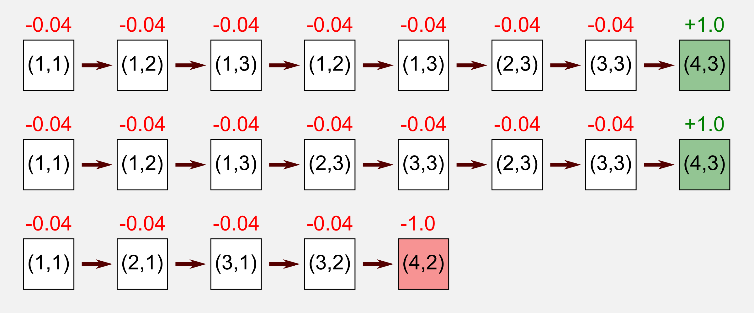
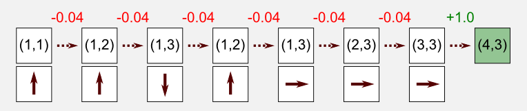
Now let’s go back to our cleaning robot and let’s see what does it mean to apply the MC method to this scenario. As usual the robot starts in state (1, 1) and it follows its internal policy. At each step it records the reward obtained and saves an history of all the states visited until reaching a terminal state. We define an episode the sequence of states from the starting state to the terminal state. Let’s suppose that our robot recorded the following three episodes:

The robot followed its internal policy but an unknown transition model perturbed the trajectory leading to undesired states. In the first and second episode, after some fluctuation the robot eventually reached the terminal state obtaining a positive reward. In the third episode the robot moved along a wrong path reaching the stairs and falling down (reward: -1.0). The following is another representation of the three episodes:

Each occurrence of a state during the episode is called visit. The concept of visit defines two different MC approaches:

1. First-Visit MC: \(U^{\pi}(s)\) is defined as the average of the returns following the first visit to \(s\) in a set of episodes.

2. Every-Visit MC: \(U^{\pi}(s)\) is defined as the average of the returns following all the visit to \(s\) in a set of episodes.

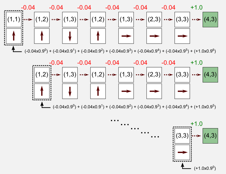
I will focus only on the First-Visit MC method in this post. What does return means? The return is the sum of discounted reward. I already presented the return in the first post when I introduced the Bellman equation and the utility of a state history.

\[\text{Return}(s) = \sum_{t=0}^{\infty} \gamma^{t} R(S_{t})\]

Nothing new. We have the discount factor \(\gamma\), the reward function \(R(s)\) and \(S_{t}\) the state reached at time \(t\). We can calculate the return for the state (1,1) of the first episode, with \(\gamma=0.9\), as follows:

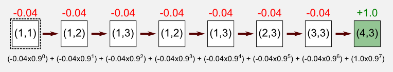
The return for the first episode is 0.27. Following the same procedure we get the same result for the second episode. For the third episode we get a different return: -0.79. After the three episodes we came out with three different returns: 0.27, 0.27, -0.79. How can we use returns to estimate utilities? I will now introduce the core equation used in the MC method, which give the utility of a state following the policy \(\pi\):

\[U^{\pi}(s) = E \Bigg[ \sum_{t=0}^{\infty} \gamma^{t} R(S_{t}) \Bigg]\]

If you compare this equation with the equation used to calculate the return you will see only one difference: to obtain the utility function we take the expectation of the returns. That’s it. To find the utility of a state we need to calculate the expectation of the returns for that state. In our example after only three episodes the approximated utility for the state (1, 1) is: (0.27+0.27-0.79)/3=-0.08. However, an estimation based only on three episodes is inaccurate. We need more episodes in order to get the true value. Why do we need more episodes?

Here the MC terminology steps into. We can define \(S_{t}\) to be a discrete random variable that can represent all the available states with a certain probability. Every time our robot enters in a state is like picking a value for the random variable \(S_{t}\). For each state of each episode we can calculate the return and store it in a list. Repeating this process for a large number of times is guaranteed to converge to the true utility. How is that possible? This is the result of a famous theorem known as the law of large number. Understanding the law of large number is crucial. Rolling a six-sided dice produces one of the numbers 1, 2, 3, 4, 5, or 6, each with equal probability. The expectation is 3.5 and can be calculated as the arithmetic mean: (1+2+3+4+5+6)/6=3.5. Using a MC approach we can obtain the same value, let’s do it in Python:

import numpy as np

# Trowing a dice for N times and evaluating the expectation
dice = np.random.randint(low=1, high=7, size=3)
print("Expectation (rolling 3 times): " + str(np.mean(dice)))
dice = np.random.randint(low=1, high=7, size=10)
print("Expectation (rolling 10 times): " + str(np.mean(dice)))
dice = np.random.randint(low=1, high=7, size=100)
print("Expectation (rolling 100 times): " + str(np.mean(dice)))
dice = np.random.randint(low=1, high=7, size=1000)
print("Expectation (rolling 1000 times): " + str(np.mean(dice)))
dice = np.random.randint(low=1, high=7, size=100000)
print("Expectation (rolling 100000 times): " + str(np.mean(dice)))

Expectation (rolling 3 times): 4.0
Expectation (rolling 10 times): 2.9
Expectation (rolling 100 times): 3.47
Expectation (rolling 1000 times): 3.481
Expectation (rolling 100000 times): 3.49948

As you can see the estimation of the expectation converges to the true value of 3.5. What we are doing in MC reinforcement learning is exactly the same but in this case we want to estimate the utility of each state based on the return of each episode. Similarly to the dice, more episodes we take into account more accurate our estimation will be.

Python implementation

As usual we will implement the algorithm in Python. I wrote a class called GridWorld contained in the module gridworld.py available in my GitHub repository. Using this class it is possible to create a grid world of any size and add obstacles and terminal states. The cleaning robot will move in the grid world following a specific policy. Let’s bring to life our 4x3 world:

import numpy as np
from gridworld import GridWorld

# Declare our environmnet variable
# The world has 3 rows and 4 columns
env = GridWorld(3, 4)
# Define the state matrix
# Adding obstacle at position (1,1)
# Adding the two terminal states
state_matrix = np.zeros((3,4))
state_matrix[0, 3] = 1
state_matrix[1, 3] = 1
state_matrix[1, 1] = -1
# Define the reward matrix
# The reward is -0.04 for all states but the terminal
reward_matrix = np.full((3,4), -0.04)
reward_matrix[0, 3] = 1
reward_matrix[1, 3] = -1
# Define the transition matrix
# For each one of the four actions there is a probability
transition_matrix = np.array([[0.8, 0.1, 0.0, 0.1],
                              [0.1, 0.8, 0.1, 0.0],
                              [0.0, 0.1, 0.8, 0.1],
                              [0.1, 0.0, 0.1, 0.8]])
# Define the policy matrix
# 0=UP, 1=RIGHT, 2=DOWN, 3=LEFT, NaN=Obstacle, -1=NoAction
# This is the optimal policy for world with reward=-0.04
policy_matrix = np.array([[1,      1,  1,  -1],
                          [0, np.NaN,  0,  -1],
                          [0,      3,  3,   3]])
# Set the matrices 
env.setStateMatrix(state_matrix)
env.setRewardMatrix(reward_matrix)
env.setTransitionMatrix(transition_matrix)

In a few lines I defined a grid world with the properties of our example. The policy is the optimal policy for a reward of -0.04 as we saw in the first post. Now, it is time to reset the environment (move the robot to starting position) and use the render() method to display the world.

#Reset the environment
observation = env.reset()
#Display the world printing on terminal
env.render()

Running the snippet above we get the following print on screen:

 -  -  -  * 
 -  #  -  * 
 ○  -  -  -

I represented free positions with - the two terminal states with * obstacles with # and the robot with ○. Now we can run an episode using a loop:

for _ in range(1000):
    action = policy_matrix[observation[0], observation[1]]
    observation, reward, done = env.step(action)
    print("")
    print("ACTION: " + str(action))
    print("REWARD: " + str(reward))
    print("DONE: " + str(done))
    env.render()
    if done: break

Given the transition matrix and the policy the most likely output of the script will be something like this:

 -  -  -  *      -  -  -  *      ○  -  -  *
 -  #  -  *      ○  #  -  *      -  #  -  *
 ○  -  -  -      -  -  -  -      -  -  -  -


 -  ○  -  *      -  -  ○  *      -  -  -  ○
 -  #  -  *      -  #  -  *      -  #  -  *
 -  -  -  -      -  -  -  -      -  -  -  -

You can find the full example in the GitHub repository. If you are familiar with OpenAI Gym you will find many similarities with my code. I used the same structure and I implemented the same methods step() reset() and render(). In particular the method step() moves forward at t+1 and returns the reward, the observation (position of the robot), and a variable called done which is True when the episode is finished (the robot reached a terminal state).

Now we have all we need to implement the MC method. Here I will use a discount factor of \(\gamma=0.999\), the best policy \(\pi^{*}\) and the same transition model used in the previous post. Remember that with the current transition model the robot will go in the desired direction only 80% of the times. First of all, I wrote a function to estimate the return:

def get_return(state_list, gamma):
    counter = 0
    return_value = 0
    for visit in state_list:
        reward = visit[1]
        return_value += reward * np.power(gamma, counter)
        counter += 1
    return return_value

The function get_return() takes as input a list containing tuples (position, reward) and the discount factor gamma, the output is a value representing the return for that action list. We are going to use the function get_return() in the following loop in order to get the returns for each episode and estimate the utilities. The following part is crucial, I added many comments to make it readable.

# Defining an empty utility matrix
utility_matrix = np.zeros((3,4))
# init with 1.0e-10 to avoid division by zero
running_mean_matrix = np.full((3,4), 1.0e-10) 
gamma = 0.999 #discount factor
tot_epoch = 50000
print_epoch = 1000

for epoch in range(tot_epoch):
    #Starting a new episode
    episode_list = list()
    #Reset and return the first observation
    observation= env.reset(exploring_start=False)
    for _ in range(1000):
        # Take the action from the action matrix
        action = policy_matrix[observation[0], observation[1]]
        # Move one step in the environment and get obs and reward
        observation, reward, done = env.step(action)
        # Append the visit in the episode list
        episode_list.append((observation, reward))
        if done: break
    # The episode is finished, now estimating the utilities
    counter = 0
    # Checkup to identify if it is the first visit to a state
    checkup_matrix = np.zeros((3,4))
    # This cycle is the implementation of First-Visit MC.
    # For each state stored in the episode list it checks if it
    # is the first visit and then estimates the return.
    for visit in episode_list:
        observation = visit[0]
        row = observation[0]
        col = observation[1]
        reward = visit[1]
        if(checkup_matrix[row, col] == 0):
            return_value = get_return(episode_list[counter:], gamma)
            running_mean_matrix[row, col] += 1
            utility_matrix[row, col] += return_value
            checkup_matrix[row, col] = 1
        counter += 1
    if(epoch % print_epoch == 0):
        print("Utility matrix after " + str(epoch+1) + " iterations:") 
        print(utility_matrix / running_mean_matrix)

#Time to check the utility matrix obtained
print("Utility matrix after " + str(tot_epoch) + " iterations:")
print(utility_matrix / running_mean_matrix)

Executing this script will print the estimation of the utility matrix every 1000 iterations:

Utility matrix after 1 iterations:
[[ 0.59184009  0.71385957  0.75461418  1.        ]
 [ 0.55124825  0.          0.87712296  0.        ]
 [ 0.510697    0.          0.          0.        ]]

Utility matrix after 1001 iterations:
[[ 0.81379324  0.87288388  0.92520101  1.        ]
 [ 0.76332603  0.          0.73812382 -1.        ]
 [ 0.70553067  0.65729802  0.          0.        ]]

Utility matrix after 2001 iterations:
[[ 0.81020502  0.87129531  0.92286107  1.        ]
 [ 0.75980199  0.          0.71287269 -1.        ]
 [ 0.70275487  0.65583747  0.          0.        ]]


...

Utility matrix after 50000 iterations:
[[ 0.80764909  0.8650596   0.91610018  1.        ]
 [ 0.7563441   0.          0.65231439 -1.        ]
 [ 0.69873614  0.6478315   0.          0.        ]]

As you can see the utility gets more and more accurate and in the limit to infinite it converges to the true values. In the first post we already found the utilities of this particular grid world using the dynamic programming techniques. Here we can compare the results obtained with MC and the ones obtained with dynamic programming:

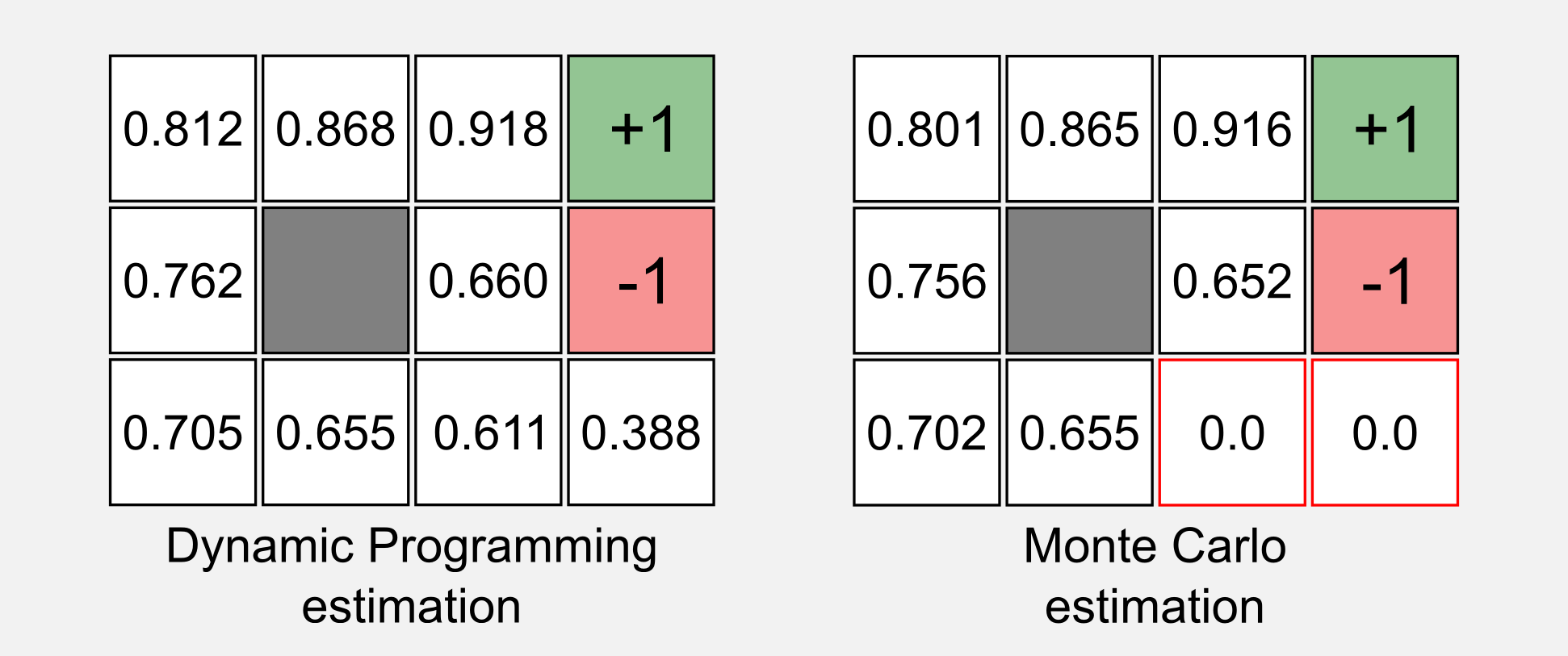
If you observe the two utility matrices you will notice many similarities but two important differences. The utility estimations for the states (4,1) and (3,1) are equal to zero. This can be considered one of the limitations and at the same time one of the advantage of MC methods. The policy we are using, the transition probabilities, and the fact that the robot always start from the same position (bottom-left corner) are responsible for the wrong estimate in those states. Starting from the state (1,1) the robot will never reach those states and it cannot estimate the corresponding utilities. As I told you this is a problem because we cannot estimate those values but at the same time it is an advantage. In a very big grid world we can estimate the utilities only for the states we are interested in, saving time and resources and focusing only on a particular subspace of the world.

What we can do to estimate the values for each state? A possible solution is called exploring starts and consists in starting from all the available states. This guarantees that all states will be visited in the limit of an infinite number of episodes. To enable the exploring starts in our code the only thing to do is to set the parameter exploring_strarts in the reset() function to True as follows:

observation = env.reset(exploring_start=True)

Now every time a new episode begins the robot will start from a random position. Running again the script will result in the following estimations:

Utility matrix after 1 iterations:
[[ 0.87712296  0.918041    0.959       1.        ]
 [ 0.83624584  0.          0.          0.        ]
 [ 0.          0.          0.          0.        ]]

Utility matrix after 1001 iterations:
[[ 0.81345829  0.8568502   0.91298468  1.        ]
 [ 0.76971062  0.          0.64240071 -1.        ]
 [ 0.71048183  0.65156625  0.62423942  0.3622782 ]]

Utility matrix after 2001 iterations:
[[ 0.80248079  0.85321     0.90835335  1.        ]
 [ 0.75558086  0.          0.64510648 -1.        ]
 [ 0.69689178  0.64712344  0.6096939   0.34484468]]

...

Utility matrix after 50000 iterations:
[[ 0.8077211   0.86449595  0.91575904  1.        ]
 [ 0.75630573  0.          0.65417382 -1.        ]
 [ 0.6989143   0.64707444  0.60495949  0.36857044]]

As you can see this time we got the right values for the states (4,1) and (3,1). Until now we assumed that we had a policy and we used that policy to estimate the utility function. What to do when we do not have a policy? In this case there are other methods we can use. Russel and Norvig called this case active reinforcement learning. Following the definition of Sutton and Barto I will call this case the model-free Monte Carlo control estimation.

Monte Carlo control

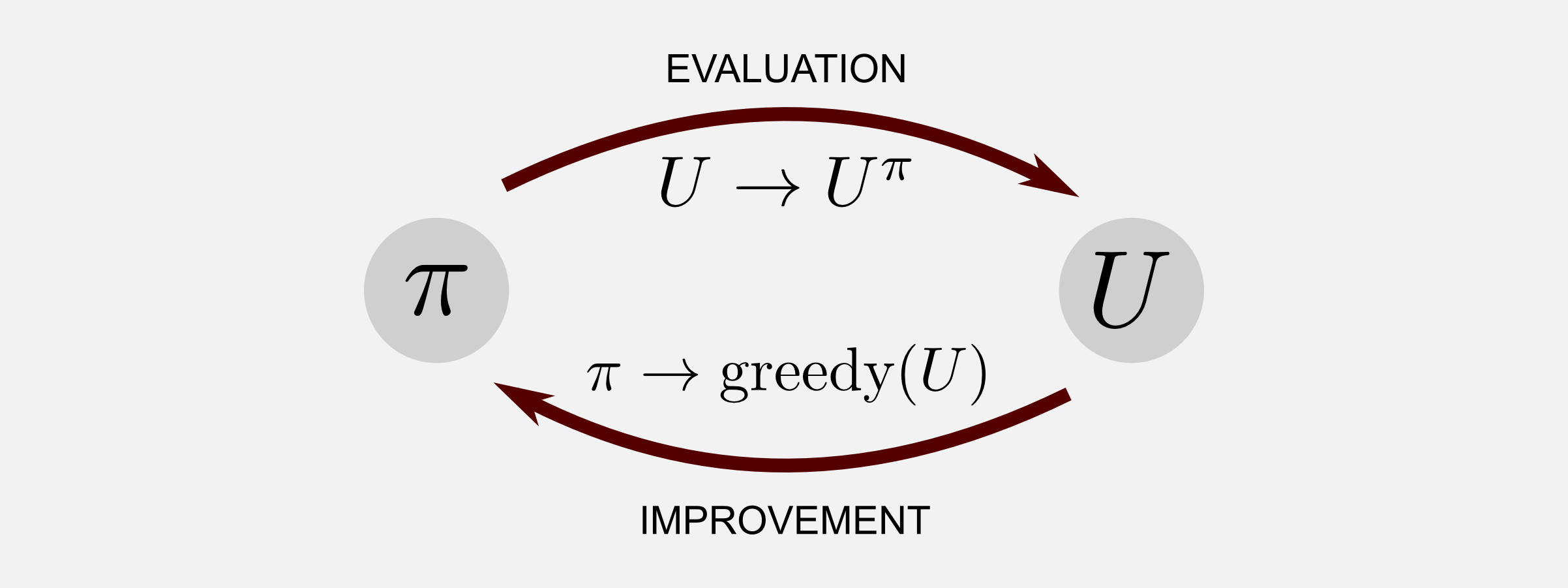
The MC methods for control (active) are slightly different from MC methods for prediction (passive). In some sense the MC control problem is more realistic because we need to estimate a policy that is not given. The mechanism behind MC for control is the same we used in the dynamic programming approach. In the Sutton and Barto book it is called Generalised Policy Iteration or GPI. The GPI is well explained by the policy iteration algorithm of the first post. The policy iteration allowed finding the utility values for each state and at the same time the optimal policy \(\pi^{*}\). The approach we used in policy iteration included two steps:

1. Policy evaluation: \(U \rightarrow U^{\pi}\)
2. Policy improvement: \(\pi \rightarrow greedy(U)\)

The first step makes the utility function consistent with the current policy (evaluation). The second step makes the policy \(\pi\) greedy with respect to the current utility function (improvement). The two changes work against each other, creating a moving target for the other, but together they collaborate making both policy and value function approach optimal.

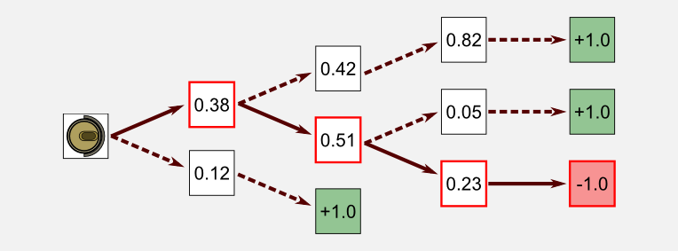
Examining the second step we notice a new term: greedy. What does it means greedy? A greedy algorithm makes the local optimal choice at each step. In our case greedy means to take for each state the action with the highest utility and update the policy with that action. However, following only local cues does not (generally) lead to optimal solutions. For example, choosing the highest utility at each step in the following case leads to a negative reward.

How can the greedy strategy work? It works because the local choice is evaluated using the utility function adjusted in time. At the beginning the agent will follow many sub-optimal paths but after a while the utilities will start to converge to the true values and the greedy strategy will lead to positive rewards. All reinforcement learning methods can be described in terms of policy iteration and more specifically in terms of GPI. Keeping the GPI idea in your mind will let you understand easily control methods. In order to fully understand the MC method for control I have to introduce another topic: the Q-function.

Action Values and the Q-function

Until now we used the function \(U\) called the utility function (aka value function, state-value function) as a way to estimate the utility (value) of a state. More precisely, we used \(U^{\pi}(s)\) to estimate the value of a state \(s\) under a policy \(\pi\). Now it’s time to introduce a new function called \(Q\) (aka action-value function) defined as follows:

\[Q^{\pi}(s, a) = E \big\{ \text{Return}_{t} | s_{t}=s, a_{t}=a \big\}\]

That’s it, the Q-function takes the action \(a\) in state \(s\) under the policy \(\pi\) and returns the utility of that state-action pair. The Q-function is defined as the expected return starting from \(s\), taking the action \(a\) and thereafter following policy \(\pi\).

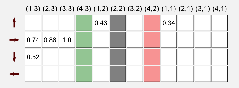
Why do we need the function Q in MC methods? In model-free reinforcement learning the utility of the states are not sufficient to suggest a policy. One must explicitly estimate the utility of each action, thus the primary goal in MC methods for control is to estimate the function \(Q^{*}\). What I said previously about the GPI applies also to the action-value function Q. Estimating the optimal action-value function is not different from estimating the utility function. The first-visit MC method for control estimation averages the return after a specific state-action pair has been visited for the first time. We must think in terms of state-action pairs and not in terms of states. When we estimated the utility function \(U\) we stored the utilities in a matrix having the same dimension of the world. Here, we need a new way to represent the state-value function Q, because we have to take into account the actions. What we can do is to have a row for each action and a column for each state. Imagine to take all the 12 states of our 4x3 grid world and dispose them along a single row, then repeat the process for all the four possible actions (up, right, down, left). The resulting (empty) matrix is the following:

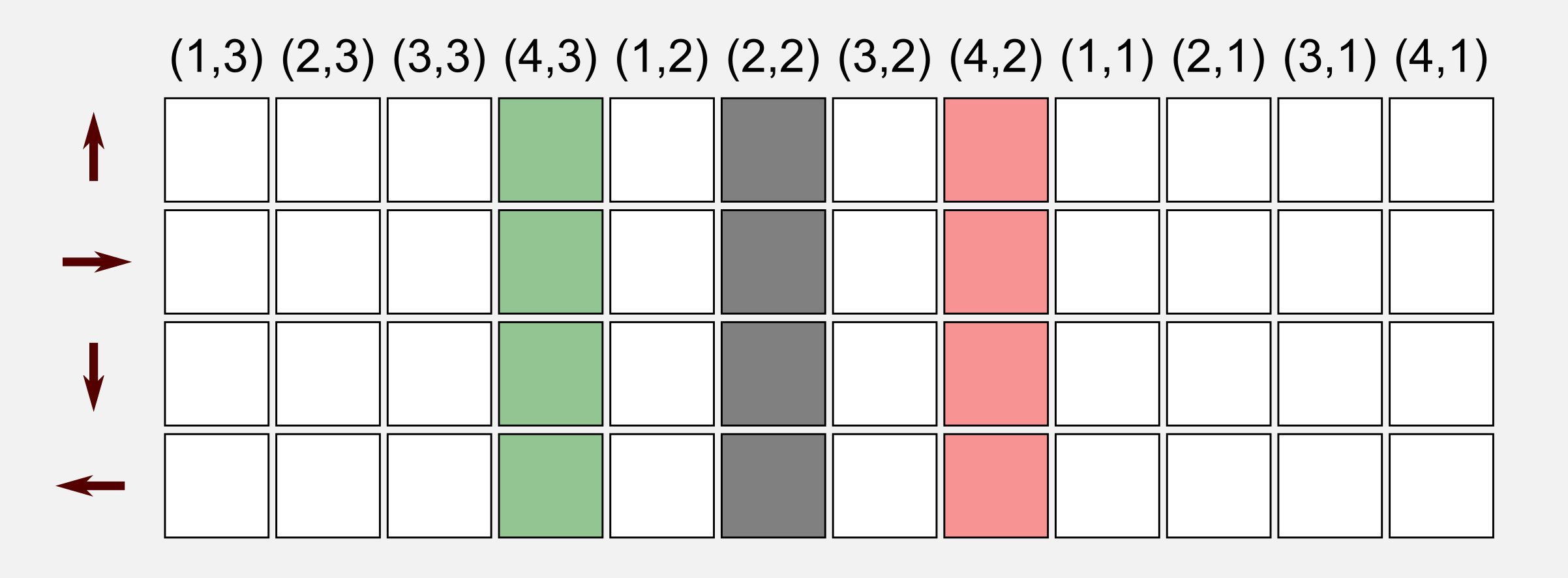
The state-action matrix stores the utilities of executing a specific action in a specific state, thus with a query to the matrix we can estimate which action should be executed in order to have the highest utility. In the MC control case we have to change our mindset when analyzing an episode. Each state has an associated action, and executing this action in that state leads to a new state and a reward. Graphically we can represent an episode pairing states with the corresponding actions:

The episode above is the same we used as example in the MC for prediction. The robot starts at (1,1) reaching the charging station after seven visits. Here, we can calculate the returns as usual. Recall that we are under the assumption of first-visit MC, and we update the entry for the state-action pair (1,2)-UP only once, since this pair is present twice in the episode. To estimate the utility we have to decompose the episode and evaluate the return that follows the first occurrence of the state-action pair. In our example, we have to compute the return for the pair (1,1)-UP, the pair (1,2)-UP, the pair (1,3)-DOWN, skip the pair (1,2)-UP (already updated), the pair (1,3)-RIGHT, etc. In the following image you can see this process and how the returns are evaluated:

After this episode the matrix containing the values for the state-action utilities can be updated. In our case the new matrix will contain the following values:

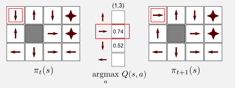
After a second episode we will fill more entries in the table. Going on in this way will eventually lead to a complete state-action table with all the entries filled. This step is what is called evaluation in the GPI framework. The second step of the algorithm is the improvement. In the improvement we take our randomly initialised policy \(\pi\) and we update it in the following way:

\[\pi(s) = \underset{a}{\text{ argmax }} Q(s,a)\]

That’s it, we are making the policy greedy choosing for each state \(s\) appearing in the episode the action with maximal Q-value. For example, if we consider the state (1,3) (top-left corner in the grid world) we can update the entry of the policy matrix taking the action with the highest value in the state-action table. In our case, after the first episode the action with the highest value is RIGHT which has a Q-value of 0.74.

In MC for control it is important to guarantee a uniform exploration of all the state-action pairs. Following the policy \(\pi\) it can happen that relevant state-action pairs are never visited. Without returns the method will not improve. The solution is to use exploring starts specifying that the first step of each episode starts at a state-action pair and that every such pair has a non-zero probability of being selected. It’s time to implement the algorithm in Python.

Python implementation

I will use again the function get_return() but this time the input will be a list containing tuples (observation, action, reward):

def get_return(state_list, gamma):
   """ Get the return for a list of action-state values.

   @return get the Return
   """ 
   counter = 0
   return_value = 0
   for visit in state_list:
      reward = visit[2]
      return_value += reward * np.power(gamma, counter)
      counter += 1
   return return_value

I will use a function called update_policy() that makes the policy greedy with respect to the current state-action function:

def update_policy(episode_list, policy_matrix, state_action_matrix):
  """ Update a policy 

  The function makes the policy greedy in respect 
  of the state-action matrix.
  @return the updated policy
  """ 
  for visit in episode_list:
    observation = visit[0]
    col = observation[1] + (observation[0]*4)
    if(policy_matrix[observation[0], observation[1]] != -1):
      policy_matrix[observation[0], observation[1]] = \
          np.argmax(state_action_matrix[:,col])
  return policy_matrix

The update_policy() function is part of the improvement step of the GPI and it is fundamental for the convergence to an optimal policy. I will also use the function print_policy(), already used in the previous post, to print the policy using the symbols: ^, >, v, <, *, #. In the main() function I initialized a random policy matrix and the state_action_matrix that contains the utilities of each state-action pair. The matrix can be initialized with zeros or random values, it does not matter.

# Random policy matrix
policy_matrix = np.random.randint(low=0, high=4, 
                                  size=(3, 4)).astype(np.float32)
policy_matrix[1,1] = np.NaN #NaN for the obstacle at (1,1)
policy_matrix[0,3] = policy_matrix[1,3] = -1 #No action (terminal states)

# State-action matrix (init to zeros or to random values)
state_action_matrix = np.random.random_sample((4,12)) # Q

Finally, the main loop of the algorithm. This is not so different from the loop used in MC prediction:

for epoch in range(tot_epoch):
# Starting a new episode
episode_list = list()
# Reset and return the first observation
observation = env.reset(exploring_starts=True)
is_starting = True
for _ in range(1000):
    # Take the action from the action matrix
    action = policy_matrix[observation[0], observation[1]]
    # If the episode just started then it is
    # necessary to choose a random action (exploring starts)
    if(is_starting): 
        action = np.random.randint(0, 4)
        is_starting = False      
    # Move one step in the environment and gets 
    # a new observation and the reward
    new_observation, reward, done = env.step(action)
    #Append the visit in the episode list
    episode_list.append((observation, action, reward))
    observation = new_observation
    if done: break
# The episode is finished, now estimating the utilities
counter = 0
# Checkup to identify if it is the first visit to a state-action
checkup_matrix = np.zeros((4,12))
# This cycle is the implementation of First-Visit MC.
# For each state-action stored in the episode list it checks if 
# it is the first visit and then estimates the return. 
# This is the Evaluation step of the GPI.
for visit in episode_list:
    observation = visit[0]
    action = visit[1]
    col = observation[1] + (observation[0]*4)
    row = action
    if(checkup_matrix[row, col] == 0):
        return_value = get_return(episode_list[counter:], gamma)
        running_mean_matrix[row, col] += 1
        state_action_matrix[row, col] += return_value
        checkup_matrix[row, col] = 1
    counter += 1
# Policy Update (Improvement)
policy_matrix = update_policy(episode_list, 
                              policy_matrix, 
                              state_action_matrix/running_mean_matrix)
# Printing
if(epoch % print_epoch == 0):
    print("")
    print("State-Action matrix after " + str(epoch+1) + " iterations:") 
    print(state_action_matrix / running_mean_matrix)
    print("Policy matrix after " + str(epoch+1) + " iterations:") 
    print(policy_matrix)
    print_policy(policy_matrix)
# Time to check the utility matrix obtained
print("Utility matrix after " + str(tot_epoch) + " iterations:")
print(state_action_matrix / running_mean_matrix)

If we compare the code below with the one used in MC for prediction we will notice some important differences, for example the following condition:

if(is_starting): 
    action = np.random.randint(0, 4)
    is_starting = False 

This condition satisfies the exploring starts. The MC algorithm will converge to the optimal solution only if we assure exploring starts. In MC for control it is not sufficient to select random starting states. During the iterations the algorithm will improve the policy only if all the actions have a non-zero probability to be chosen. In this sense when the episode starts we have to select a random action, this must be done only for the starting state.

There is another subtle difference. In the code I differentiate between observation and new_observation, the observation at time \(t\) and the observation at time \(t+1\). What we need to store in our episode list is the observation at \(t\), the action taken at \(t\) and the reward obtained at \(t+1\). Remember that we are interested in the utility of taking a certain action in a certain state.

It is time to run the script. Before recall that for the simple 4x3 gridworld we already know the optimal policy. In the first post we have found the optimal policy with a reward equal to -0.04 (for non terminal states) and with transition model having 80-10-10 percent probabilities. The optimal policy is the following:

Optimal policy:

 >   >   >   * 
 ^   #   ^   * 
 ^   <   <   < 

In the optimal policy the robot will move far away from the stairs at state (4, 2) and will reach the charging station through the longest path. Now, I will show you the evolution of the policy once we run the script for MC control estimation:

Policy after 1 iterations:
 ^   >   v   * 
 <   #   v   * 
 v   >   <   >

...

Policy after 3001 iterations:
 >   >   >   * 
 >   #   ^   * 
 >   >   ^   < 

...

Policy after 78001 iterations:
 >   >   >   * 
 ^   #   ^   * 
 ^   <   ^   <

...

Policy after 405001 iterations:
 >   >   >   * 
 ^   #   ^   * 
 ^   <   <   <

...

Policy after 500000 iterations:
 >   >   >   * 
 ^   #   ^   * 
 ^   <   <   < 

At the beginning the MC method is initialized with a random policy, therefore it is not a surprise that the first policy is a complete non-sense. After 3000 iteration the algorithm finds a sub-optimal policy. In this policy the robot moves close to the stairs in order to reach the charging station. As we said in the previous post this is risky because the robot can fall down. At iteration 78000 the algorithm finds another policy, that is still sub-optimal but slightly better than the previous one. Finally at iteration 405000 the algorithm finds the optimal policy and stick to it until the end.

The MC method cannot converge to any sub-optimal policy. From the GPI point of view this is obvious. If the algorithm converges to a sub-optimal policy then the utility function would eventually converge to the utility function for that policy causing the policy to change. Stability is reached only when both the policy and the utility function are optimal. Convergence to this optimal fixed point seems inevitable but has not yet been formally proved.

Conclusions

I would like to reflect for a moment on the beauty of the MC algorithm. In MC for control the method can estimate the best policy from nothing. The robot is moving in the environment trying different actions and following the consequences of those actions until the end. That’s all. The robot does not know the reward function, it does not know the transition model and it does not have any policy to follow. Nevertheless the algorithm improves until reaching the optimal strategy.

Be careful MC methods are not perfect. The fact that we have to save a full episode before updating the utility function is a strong limitation. It means that if you want to train a robot for driving a car you should wait until the robot crashes into a wall in order to update the policy. To overcome this problem we can use another algorithm called Temporal Differencing (TD) learning. Using TD methods we can obtain the same result of MC methods but we can update the utility function after a single step. In the next post I will introduce TD methods, the foundations of Q-Learning and Deep Reinforcement Learning.

Index

1. [First Post] Markov Decision Process, Bellman Equation, Value iteration and Policy Iteration algorithms.
2. [Second Post] Monte Carlo Intuition, Monte Carlo methods, Prediction and Control, Generalised Policy Iteration, Q-function.
3. [Third Post] Temporal Differencing intuition, Animal Learning, TD(0), TD(λ) and Eligibility Traces, SARSA, Q-learning.
4. [Fourth Post] Neurobiology behind Actor-Critic methods, computational Actor-Critic methods, Actor-only and Critic-only methods.
5. [Fifth Post] Evolutionary Algorithms introduction, Genetic Algorithms in Reinforcement Learning, Genetic Algorithms for policy selection.
6. [Sixt Post] Reinforcement learning applications, Multi-Armed Bandit, Mountain Car, Inverted Pendulum, Drone landing, Hard problems.
7. [Seventh Post] Function approximation, Intuition, Linear approximator, Applications, High-order approximators.
8. [Eighth Post] Non-linear function approximation, Perceptron, Multi Layer Perceptron, Applications, Policy Gradient.

Resources

• The complete code for MC prediction and MC control is available on the dissecting-reinforcement-learning official repository on GitHub.

• Dadid Silver’s course (DeepMind) in particular lesson 4 [pdf][video] and lesson 5 [pdf][video].

• Artificial intelligence: a modern approach. (chapters 17 and 21) Russell, S. J., Norvig, P., Canny, J. F., Malik, J. M., & Edwards, D. D. (2003). Upper Saddle River: Prentice hall. [web] [github]

• Reinforcement learning: An introduction. Sutton, R. S., & Barto, A. G. (1998). Cambridge: MIT press. [html]

• Reinforcement learning: An introduction (second edition). Sutton, R. S., & Barto, A. G. (2018). [pdf]

References

Russell, S. J., Norvig, P., Canny, J. F., Malik, J. M., & Edwards, D. D. (2003). Artificial intelligence: a modern approach (Vol. 2). Upper Saddle River: Prentice hall.

Sutton, R. S., & Barto, A. G. (1998). Reinforcement learning: An introduction (Vol. 1, No. 1). Cambridge: MIT press.