Dissecting Reinforcement Learning-Part.6

Hello folks! Welcome to the sixth episode of the “Dissecting Reinforcement Learning” series. Until now we saw how reinforcement learning works. However we applied most of the techniques to the robot cleaning example. I decided to follow this approach because I think that the same example applied to different techniques can help the reader to better understand what changes from one scenario to the other. Now it is time to apply this knowledge to other problems. In each one of the following sections I will introduce a reinforcement learning problem and I will show you how to tackle it. First of all I will explaining the history behind the application, then I will implement it in Python and I will apply a reinforcement learning technique to solve it. I will follow an incremental approach, starting from the simplest case and arriving to the most complicated one. Here we are going to use a discrete representation for both the utility and the action-value function, meaning that I will represent these functions with a matrix (or look-up table if you prefer). The discretization is the only method we can use at this point in the series. In the next post I am going to introduce function approximation which is a powerful tool for dealing with complex problems.

The references for this post are the Sutton and Barto’s book (chapter 11, case studies), and “Statistical Reinforcement Learning” by Masashi Sugiyama which contains a good description of some of the applications we are going to encounter. In this post I want you to get your hands dirty! There is a lot of code to run, parameters to change and graphs to plot. You should learn by doing. Fork the Github repository if you have a Github account, or download the latest zip archive from here if you haven’t.

Multi-Armed Bandit

An armed bandit is a fancy way to call slot machines in Las Vegas. They are bandits because they steal your money! In 1950s Mosteller and Bush were studying the effect of reward on mice in a T-maze. In order to compare the performance with humans they realised a two-armed bandit experiment. The subjects could choose to pull the left or right arm in order to receive a reward. One of the two arm was more generous.

In this experiment the subject has to find a good balance between exploration and exploitation. Let’s suppose the subject plays a single round finding out that the left arm is more generous. How to proceed? You must remember that the machines are stochastic and the best one may not return the prize for a while in a short sequence. Should the subject explore the option that looks inferior or exploit the current best option? Formally we can define this problem as a Markov decision process with a single state (see the first post). There are \(N\) arms which is possible to pull and each one as a certain probability of returning a prize. We have a single state and \(N\) possible actions (one action for each arm). At each round the agent chooses one arm to pull and it receives a reward. The goal of the agent is to maximise the reward. During the years have been proposed many solutions to the multi-armed bandit problem. In the following part of the post I will show you some of these solutions, and I will show you empirically the results obtained from each one.

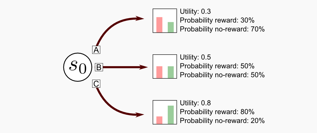
I will consider the case were \(N=3\) meaning that we have 3 possible actions (3 arms). I will call this example a three-armed testbed. A similar case has been considered by Sutton and Barto in chapter 2.1 of their book, however they used a 10-armed bandit and a Gaussian distribution to model the reward function. Here I will use a Bernoulli distribution, meaning that the rewards are either 0 or 1. From the initial state \(s_{0}\) we can choose one of three arms (A, B, C). The first arm (A) return a positive reward of 1 with 30% probability, and it returns 0 with 70% probability. The second arm (B) returns a positive reward in 50% of the cases. The third arm (C) returns a positive reward with 80% probability. The utility of each action is: 0.3, 0.5, 0.8. The utility can be estimated at runtime using an action-utility (or action-value) method. If the action \(a\) has been chosen \(k_{a}\) times leading to a series of reward \(r_{1}, r_{2},...,r_{k_{a}}\) then the utility of this specific action can be estimated through:

\[Q(a) = \frac{r_{1}, r_{2},...,r_{k_{a}}}{k_{a}}\]

It is helpful to play with this example and try different strategies. Before playing we need a way to measure exploration and exploitation. In the next sections I will quantify exploitation using the average cumulated reward and exploration using the Root Mean Square Error (RMSE) between the true utility distribution and the average estimation. When both the RMSE and the average cumulated reward are low, the agent is using an exploration-based strategy. On the other hand, when the RMSE and the average cumulated reward are high, the agent is using an exploitation-based strategy. To simplify our lives I created a Python module called multi_armed_bandit.py which has a class called MultiArmedBandit. The only parameter that must be passed to the object is a list containing the probability \(\in [0,1]\) of obtaining a positive reward:

from multi_armed_bandit import MultiArmedBandit

# Creating a bandit with 3 arms
my_bandit = MultiArmedBandit(reward_probability_list=[0.3, 0.5, 0.8])

The step() method takes as input an action which represent the index of the arm that must be pulled. For instance calling my_bandit.step(action=0) will pull the first arm, and calling my_bandit.step(action=2) will pull the third. The step() method returns the reward obtained pulling that arm, which can be 1 or 0. The method does not return anything else. Remember that we are not moving here. There is no point in returning the state at t+1 or a variable which identifies a terminal state, because as I said the multi-armed bandit has a single state. Now it is time to play! In the next sub-sections I will show you some of the strategies that is possible to use in the three-armed testbed.

Omniscient: the word omniscient derives from Medieval Latin and it means all-knowing. An omniscient agent knows the utility distribution before playing and it follows an optimal policy. Let’s suppose that you work for the company that is producing the three-armed bandit. Your duty is to realise the firmware of the machine. Since you are the designer you perfectly know the probability of a positive reward for each one of the three arms. It’s time for vacation and you decide to go to Las Vegas. You enter in a Casino and you see just in front of you the particular machine you worked on. What are you gonna do? Probably you will start pulling the third arm (C) like a crazy until your pockets are full of coins. You know that the best thing to do is to focus on the third arm because it has 80% probability of returning a positive reward. Now let’s suppose that the omniscient agent plays for 1000 rounds, what’s the cumulated reward obtained in the end? If the third arm has 80% probability of obtaining a coin we can say that after 1000 round the player will get approximately 800 coins. Keep in mind this value because it is the upper boundary for the comparison.

Random: the most intuitive strategy is a random strategy. Just pull any arm with the same probability. This is the strategy of a naive gambler. Let’s see what a random agent will obtain playing this way. We can create a random agent in a few line of code:

from multi_armed_bandit import MultiArmedBandit
import numpy as np

my_bandit = MultiArmedBandit(reward_probability_list=[0.3, 0.5, 0.8])
tot_arms = 3
tot_steps = 1000
cumulated_reward = 0
print("Starting random agent...")
for step in range(tot_steps):
    action = np.random.randint(low=0, high=tot_arms)
    reward = my_bandit.step(action)
    cumulated_reward += reward
print("Cumulated Reward: " + str(cumulated_reward))

Running the script will pull the arms 1000 times, and the reward obtained will be accumulated in the variable called cumulated_reward. I run the script several times (it takes just a few milliseconds) and I obtained cumulated rewards of 527, 551, 533, 511, 538, 540. Here I want you to reason on what we got. Why all the cumulated rewards oscillate around a value of 530? The random agent pulled the arms with (approximately) the same probability, meaning that it pulled the first arm 1/3 of the times, the second arm 1/3 of the times, and the third arm 1/3 of the times. The final score can be approximated as follows: 300/3 + 500/3 + 800/3 = 533.3. Remember that the process is stochastic and we can have a small fluctuation every time. To neutralise this fluctuation I introduced another loop of 2000 iterations, which repeats the script 2000 times.

Average Cumulated Reward: 533.441
Average utility distribution: [0.29912987  0.50015673  0.80060398]
Average utility RMSE: 0.000618189621201

The average value for the cumulated reward is 533.4, which is very close to the estimation we made. At the same time the RMSE is extremely low (0.0006) meaning that the random agent is greatly unbalanced in direction of exploration instead of exploitation. The complete code is in the official repository and is called random_agent_bandit.py.

Greedy: the agent that is following a greedy strategy pulls all the arms in the first turn, then it selects the arm that returned the highest reward. This strategy do not really encourage exploration and this is not surprising. We have already seen in the second post that a greedy strategy should be part of a larger Generalised Policy Iteration (GPI) scheme in order to converge. Only with constant updates of the utility function it is possible to improve the policy. An agent that uses a greedy strategy can be fooled by random fluctuations and it can think that the second arm is the best one only because in a short series it returned more coins. Running the script for 2000 episodes, each one having 1000 rounds, we get:

Average cumulated reward: 733.153
Average utility distribution: [0.14215225  0.2743839   0.66385142]
Average utility RMSE: 0.177346151284

The result on our test is 733 which is significantly over the random score. We said that the true utility distribution is [0.3, 0.5, 0.8]. The greedy agent has an average utility distribution of [0.14, 0.27, 0.66] and a RMSE of 0.18, meaning that it underestimates the utilities because of its blind strategy which does not encourage exploration. Here we can see an inverse pattern respect to the random agent, meaning that for the greedy player both the average reward and the RMSE are high.

Epsilon-greedy: we already encountered this strategy. At each time step the agent is going to select the most generous arm with probability \(p = 1 - \epsilon\) (exploitation) and it will randomly choose one of the other arms with probability \(q = \epsilon\) (exploration). A value which is often choose for epsilon is \(\epsilon = 0.1\). I created a script for testing this agent that you will find on the official repository and is called epsilon_greedy_agent_bandit.py. Using a value of epsilon equal to 0.1, and running the script for 1000 steps and 2000 episodes I got the following results:

Average cumulated reward: 763.802
Average utility distribution: [0.2934227   0.49422608  0.80003897]
Average utility RMSE: 0.00505307354513

The average cumulated reward is 763 which is higher than the random and the greedy agents. The random exploration helps the agent to converge closely to the true utility distribution leading to a low RMSE (0.005).

Softmax-greedy: in the epsilon-greedy strategy the action is sampled randomly from a uniform distribution. The softmax sampling goes a step further and chose with higher probability those actions that lead to more reward. We already used a softmax strategy in the fourth post when talking about actor-critic methods. This strategy takes its name from the softmax function, which can be easily implemented in Python:

def softmax(x):
    """Compute softmax distribution of array x.

    @param x the input array
    @return the softmax array
    """
    return np.exp(x - np.max(x)) / np.sum(np.exp(x - np.max(x)))

In the softmax-greedy stategy we select the most generous arm with probability \(p = \sigma\) and one of the other arms (using softmax sampling) with probability \(q = 1 - \sigma\). The effect of this sampling is to select actions based on the utility distribution which has been estimated until that point. If the third arm has an higher chance of giving a reward then the softmax-greedy agent will choose that arm more frequently when a random action has to be selected. Running the python script with sigma=0.1 we get the following outcome:

Average cumulated reward: 767.249
Average utility distribution: [0.29169784  0.49047397  0.79968229]
Average utility RMSE: 0.00729776356239

The result of 767 is slightly higher than epsilon-greedy, but at the same time also the RMSE error is slightly higher. Increasing exploitation we decreased exploration. As you can see there is a delicate balance between exploration and exploitation and it is not so straightforward to find the right trade-off. The complete code is included in the repository and is called softmax_agent.py.

Epsilon-decreasing: when in the epsilon-greedy algorithm we had to choose a random action, we used a fixed epsilon value of 0.1. However is not always a good choice, because after many round we have a more accurate estimation of the utility distribution and we could reduce the exploration. In the decreasing strategy we set \(\epsilon = 0.1\) at the beginning and then we decrease it linearly during the game. In this way the agent will explore a lot at the beginning and it will focus on the most generous arm in the end. The script epsilon_decresing_agent_bandit.py run the strategy with a linearly decreasing epsilon that starts at 0.1 and reach 0.0001 at the last step of the episode. The results running the script is:

Average cumulated reward: 777.423
Average utility distribution: [0.28969042  0.48967624  0.80007298]
Average utility RMSE: 0.00842363169768

The average cumulated reward is 777 which is higher that the scores obtained with the previous strategies. At the same time the utility distribution is close to the original but the RMSE (0.008) is slightly higher compared to the epsilon-greedy (0.005). Once again we can notice how delicate is the balance between exploration and exploitation.

Boltzmann sampling: this strategy is based on a softmax function and for this reason it is said to be part of the sofmax action selection rules. In the softmax sampling actions that lead to more reward are sampled with an higher probability. In Boltzmann sampling the softmax function is used in order to estimate the probability \(P(a)\) of a specific action \(a\) based on the probability of the other \(N\) actions, as follows:

\[P(a) = \frac{e^{Q(a) / \tau}}{\sum_{b=1}^{N} e^{Q(b) / \tau}}\]

where \(\tau > 0\) is a parameter called temperature. High temperatures generate a distribution where all the actions have approximately the same probability to be sampled, whereas in the limit of \(\tau \rightarrow 0\) the action selection becomes greedy. We can easily implement Boltzmann sampling in python:

def boltzmann(x, temperature):
    """Compute boltzmann distribution of array x.

    @param x the input array
    @param temperature
    @return the boltzmann array
    """
    exponent = np.true_divide(x - np.max(x), temperature)
    return np.exp(exponent) / np.sum(np.exp(exponent))

The function boltzmann() takes in input an array and the temperature, and returns the Boltzmann distribution of that array. Once we have the Boltzmann distribution we can use the Numpy method numpy.random.choice() to sample an action. The complete script is called boltzmann_agent_bandit.py and is in the official repository of the project. Running the script with \(\tau\) decreased linearly from 10 to 0.01 leads to the following result:

Average cumulated reward: 648.0975
Average utility distribution: [0.29889418  0.49732589  0.79993241]
Average utility RMSE: 0.0016711564118

The strategy reached a score of 648 which is the lowest score obtained so far, but the RMSE on the utility distribution is the lowest as well (0.002). Changing the temperature decay we can see how the performance increases. Starting form a value of 0.5 and decreasing to 0.0001 we get the following results:

Average cumulated reward: 703.271
Average utility distribution: [0.29482691  0.496563    0.79982371]
Average utility RMSE: 0.00358724122464

As you can see there is a significant increase in the cumulated reward, but at the same time an increase in the RMSE. As usual, we have to find the right balance. Let’s try now with an initial temperature of 0.1 and let’s decrease it to 0.0001:

Average cumulated reward: 731.722
Average utility distribution: [0.07524908  0.18915708  0.64208991]
Average utility RMSE: 0.239493838117

We obtained a score of 732 and RMSE of 0.24 which are very close to the score of the greedy agent (reward=733, RMSE=0.18). This is not surprising because as I said previously in the limit of \(\tau \rightarrow 0\) the action selection becomes greedy. The Boltzmann sampling guarantees a wide exploration which may be extremely useful in large state spaces, however it may have some drawbacks. It is generally easy to choose a value for \(\epsilon\) in the epsilon-based strategies, but we cannot say the same for \(\tau\). Setting \(\tau\) may require a fine hand tuning which is not always possible in some problems. I suggest you to run the script with different temperature values to see the difference.

Thompson sampling: to understand this strategy it is necessary some knowledge of probability theory and Bayesian statistics. In particular you should know the most common probability distributions, and how Bayes’ theorem works. In the softmax-based approaches we estimated the reward probability using a frequentist approach. Taking into account the number of successes and failures obtained pulling each arm, we approximated the utility function. What is the utility function from a statistical point of view? The utility function is an approximation of the Bernoulli reward distributions associated with the bandit arms. In a frequentist setting the Bernoulli distribution is estimated through Maximum Likelihood Estimation (MLE) as follows:

\[P(q) = \frac{s}{s + f}\]

where \(P(q)\) is the probability of a positive reward for a specific arm, \(s\) is the number of successes, and \(f\) is the number of failures. You should notice a similarity between this equation and the Q-function we defined at the beginning. Using MLE is not the best approach because it raises a problem when there are a few samples. Let’s suppose we pulled the first arm (A) two times, and we got two positive rewards. In this case we have \(s=2\) and \(f=0\) leading to \(P(q) = 1\). This estimation is completely wrong. We know that the first arm returns a positive reward with 30% probability, our estimation says it returns a positive reward with 100% probability. In the Boltzmann sampling we partially neutralised this error using the temperature parameter, however the bias could have an effect on the final score. We should find a way to do an optimal estimation of the Bernoulli distribution based on the current data available. Using a Bayesian approach it is possible to define a prior distribution on the parameters of the reward distribution of every arm, and sample an action according to the posterior probability of being the best action. This approach is called Thompson sampling and was published by William Thompson in 1993. In the three-armed bandit testbed I defined the bandit as a Bernoulli bandit, meaning that the reward given by each arm is obtained through a Bernoulli distribution. Each arm can return a positive reward with probability of success \(q\) and probability of failure \(1-q\). By definition the Bernoulli distribution describes the binary outcome of a single experiment, for example a single coin toss (0=tail, 1=head). Here we are interested in finding another distribution, meaning \(P(q \vert s,f)\), which is called posterior in the Bayesian terminology. Knowing the posterior we know which arm returns the highest reward and we can play like an omniscient agent. Here we must be careful, the posterior is not a Bernoulli distribution, because it takes into account \(s\) and \(f\) which are the success/failure rates on a series of experiments. Which kind of distribution is it? How can we find it? We can use the Bayes’ theorem. Using this theorem we can do an optimal approximation of the posterior based on the data collected in the previous rounds. Here I define \(s\) and \(f\) as the number of successes and failures accumulated in previous trials for a specific arm, and \(q\) as the probability of obtaining a positive reward pulling that arm. The posterior can be estimated through Bayes’ theorem as follows:

\[P(q \vert s,f) = \frac{P(s,f \vert q)P(q)}{\int{}{} P(s,f \vert q) P(q) dx}\]

From this equation it is clear that for finding the posterior we need the term \(P(s,f \vert q)\) (likelihood), and the term \(P(q)\) (prior). Let’s start from the likelihood. As I said the Bernoulli distribution represents the outcome of a single experiment. In order to represent the outcome of multiple independent experiments we have to use the Binomial distribution. This distribution can tell us what is the probability of having \(s\) successes in \(s + f\) trials. The distribution is represented as follows:

\[P(s,f \vert q) = \binom{s+f}{s} q^{s} (1-q)^{f}\]

Great, we got the first missing term. Now we have to find the prior. Fortunately the Bernoulli distribution has a conjugate prior which is the Beta distribution:

\[P(q) = \frac{q^{\alpha-1} (1 - q)^{\beta - 1}}{B(\alpha, \beta)}\]

where \(\alpha, \beta > 0\) are parameters representing the success and failure rate, and \(B\) is a normalization constant (Beta function) which ensures that the probability integrates to 1. Now we have all the missing terms. Going back to the Bayes’ theorem, we can plug the Binomial distribution in place of the likelihood, and the Beta distribution in place of the prior. After some reductions we come out with the following result:

\[P(q \vert s,f) = \frac{q^{s+ \alpha-1} (1-q)^{f+ \beta-1}}{B(s+ \alpha, f+ \beta))}\]

If you give a look to the result you will notice that our posterior is another Beta distribution. That’s a really clean solution to our problem. In order to obtain the probability of a positive reward for a given arm, we simply have to plug the parameters \((\alpha + s, \beta + f)\) into a Beta distribution. The main advantage of this approach is that we are going to have better estimates of the posterior when the number of successes and failures increases. For example, let’s say that we start with \(\alpha = \beta = 1\) meaning that we suppose a uniform distribution for the prior. That’s reasonable because we do not have any previous knowledge about the arm. Let’s suppose we pull the arm three times and we obtain two successes and one failure, we can obtain the estimation of the Bernoulli distribution for that arm through \(Beta(\alpha + 2, \beta + 1)\). This is the best estimation we can do after three rounds. As we keep playing the posterior will get more and more accurate. Thompson sampling can be used also with non-Bernoulli distributions. If the reward is modelled by a multinomial distribution we can use the Dirichlet distribuion as conjugate. If the reward is modelled as Gaussian distribution we can use the Gaussian itself as conjugate.

In python we can easily implement the Thompson agent for the three-armed bandit testbed. It is necessary to keep a record of successes and failures in two Numpy arrays. Those arrays are passed to the following function:

def return_thompson_action(success_counter_array, failure_counter_array):
    """Return an action using Thompson sampling

    @param success_counter_array (alpha) success rate for each action
    @param failure_counter_array (beta) failure rate for each action
    @return the action selected
    """
    beta_sampling_array = np.random.beta(success_counter_array, 
                                         failure_counter_array)
    return np.argmax(beta_sampling_array)

Numpy implements the method numpy.random.beta() which takes in input the two arrays (\(\alpha+s, \beta+f\)) and returns an array containing the values sampled from the underlying Beta distributions. Once we have this array we only have to take the action with the highest value using np.argmax(), which corresponds to the arm with the highest probability of reward. Running the script thompson_agent_bandit.py we get the following results:

Average cumulated reward: 791.21
Average utility distribution: [0.39188487  0.50654831  0.80154085]
Average utility RMSE: 0.0531917417346

The average cumulated reward obtained is 791 which is the highest score reached so far, and it is very close to the optimal strategy of the omniscient player. At the same time the RMSE (0.05) on the utility distribution is fairly low. Thompson sampling seems to be the perfect strategy for balancing exploration and exploitation, however there are some drawbacks. In our example we used a Bernoulli distribution as posterior, but it was an oversimplification. It can be difficult to approximate the posterior distribution when the underlying function is completely unknown, moreover the evaluation of the posterior requires an integration which may be computationally expensive.

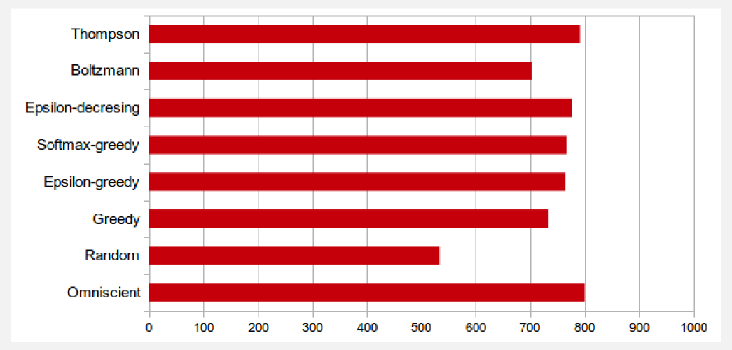
Comparing the results of the different strategies on a barchart we can see at a glance the performances obtained. Thompson sampling seems to be the best strategy in term of score, but in practical terms it is difficult to apply. Softmax-greedy and epsilon-greedy are pretty similar, and choosing the one or the other depends how much you want to encourage exploration. The epsilong-decreesing strategy is most of the time a secure choice, since it has been widely adopted and it has a clear dynamic on a wide variety of cases. For instance, modern approaches (e.g. DQN, Double DQN, etc.) use epsilon-based strategies. The homework for this section is to increase the number of arms and run the algorithms to see which one performs better. To change the number of arms you simply have to modify the very first line in main function:

reward_distribution = [0.3, 0.5, 0.8]

To generate a 10-armed bandit you can modify the variable in this way:

reward_distribution = [0.7, 0.4, 0.6, 0.1, 0.8, 0.05, 0.2, 0.3, 0.9, 0.1]

Once you have a new distribution you can run the script and register the performances of each strategy. Increasing the number of arms should make the exploration more important. A larger state space requires more exploration in order to get an higher reward.

In this section we saw how exploration can affect the results in a simple three-armed testbed. Multi-armed bandit problems are in our daily life. The doctor who has to choose the best treatment for a patient, the web-designer who has to find the best template for maximising the AdSense clicks, or the entrepreneur who has to decide how to manage budget for maximising the incomes. Now you know some strategies for dealing with these problems. In the next section I will introduce the mountain car problem, and I will show you how to use reinforcement learning to tackle it.

Mountain Car

The mountain car is a classic reinforcement learning problem. This problem was first described by Andrew Moore in his PhD thesis and is defined as follows: a mountain car is moving on a two-hills landscape. The engine of the car does not have enough power to cross a steep climb. The driver has to find a way to reach the top of the hill.

A good explanation of the probelm is presented in chapter 4.5.2 of Sugiyama’s book. I will follow the same mathematical convention here. The state space is defined by the position \(x\) obtained through the function \(sin(3x)\) in the domain [-1.2, +0.5] (\(m\)) and the velocity \(\dot{x}\) defined in the interval [-1.5, +1.5] (\(m/s\)). There are three possible actions \(a =\) [-2.0, 0.0, +2.0] which are the values of the force applied to the car (left, no-op, right). The reward obtained is positive 1.0 only if the car reaches the goal. A negative cost of living of -0.01 is applied at every time step. The mass of the car is \(m = 0.2 \ kg\), the gravity is \(g = 9.8 \ m/s^2\), the friction is defined by \(k = 0.3 \ N\), and the time step is \(\Delta t =0.1 \ s\). Given all these parameters the position and velocity of the car at \(t+1\) are updated using the following equations:

\[x_{t+1} = x_{t} + \dot{x}_{t+1} \Delta t\] \[\dot{x}_{t+1} = \dot{x}_{t} + (g \ m \ cos(3x_{t}) + \frac{a_{t}}{m} - k \ \dot{x}_{t}) \Delta t\]

The mountain car environment has been implemented in OpenAI Gym, however here I will build everything from scratch for pedagogical reason. In the repository you will find the file mountain_car.py which contains a class called MountainCar. I built this class using only Numpy and matplotlib. The class contains methods which are similar to the one used in OpenAI Gym. The main method is called step() and allows executing an action in the environment. This method returns the state at t+1 the reward and a value called done which is True if the car reach the goal. The method contains the implementations of the equation of motion and it uses the parameters previously defined.

def step(self, action):
    """Perform one step in the environment following the action.
        
    @param action: an integer representing one of three actions [0, 1, 2]
     where 0=move_left, 1=do_not_move, 2=move_right
    @return: (postion_t1, velocity_t1), reward, done
     where reward is always negative but when the goal is reached
     done is True when the goal is reached
    """
    if(action >= 3):
        raise ValueError("[MOUNTAIN CAR][ERROR] The action value "
                         + str(action) + " is out of range.")
    done = False
    reward = -0.01
    action_list = [-0.2, 0, +0.2]
    action_t = action_list[action]
    velocity_t1 = self.velocity_t + \
                  (-self.gravity * self.mass * np.cos(3*self.position_t)
                   + (action_t/self.mass) 
                   - (self.friction*self.velocity_t)) * self.delta_t
    position_t1 = self.position_t + (velocity_t1 * self.delta_t)
    # Check the limit condition (car outside frame)
    if position_t1 < -1.2:
        position_t1 = -1.2
        velocity_t1 = 0
    # Assign the new position and velocity
    self.position_t = position_t1
    self.velocity_t= velocity_t1
    self.position_list.append(position_t1)
    # Reward and done when the car reaches the goal
    if position_t1 >= 0.5:
        reward = +1.0
        done = True
    # Return state_t1, reward, done
    return [position_t1, velocity_t1], reward, done

In the object initialisation it is possible to define different parameters for the simulation. Here I will define a new car object setting the parameters we want:

from mountain_car import MountainCar

my_car = MountainCar(mass=0.2, friction=0.3, delta_t=0.1)

I added an useful method called render() which can save the episode animation in a gif or a video (it requires imagemagick and avconv). This method can be called every k episodes in order to save the animation and check the improvements. For example, to save an mp4 video it is possible to call the method with the following parameters:

my_car.render(file_path='./mountain_car.mp4', mode='mp4')

If you want an animated gif instead you can call the method in this way:

my_car.render(file_path='./mountain_car.gif', mode='gif')

Now let’s try to use the class and let’s build an agent which uses a random policy for choosing the actions. Here I will use a time step of 0.1 seconds and a total of 100 steps (which means a 10 seconds long episode). The code is very compact, and at this point of the series you can easily understand it without any additional comment:

from mountain_car import MountainCar
import random

my_car = MountainCar(mass=0.2, friction=0.3, delta_t=0.1)
cumulated_reward = 0
print("Starting random agent...")
for step in range(100):
    action = random.randint(a=0, b=2)
    observation, reward, done = my_car.step(action)
    cumulated_reward += reward
    if done: break
print("Finished after: " + str(step+1) + " steps")
print("Cumulated Reward: " + str(cumulated_reward))
print("Saving the gif in: ./mountain_car.gif")
my_car.render(file_path='./mountain_car.gif', mode='gif')
print("Complete!")

Observing the behaviour of the car in the animation generated by the script it is possible to see how difficult is the task. Using a purely random policy the car remains at the bottom of the valley and it does not reach the goal. The optimal policy is to move on the left accumulating inertia and then to push as much as possible to the right.

How can we deal with this problem using a discrete approach? We said that the state space is continuous, meaning that we have infinite values to take into account. What we can do is dividing the continuous state-action space in chunks. This is called discretization. If the car moves in a continuous space enclosed in the range \([-1.2, 0.5]\) it is possible to create 10 bins to represent the position. When the car is at -1.10 it is in the first bin, when at -0.9 in the second, etc.

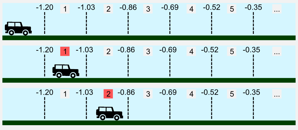
In our case both position and velocity must be discretized and for this reason we need two arrays to store all the states. Here I call bins the discrete containers (entry of the array) where both position and velocity are stored. In Numpy is easy to create these containers using the numpy.linspace() function. The two arrays can be used to define a policy matrix. In the script I defined the policy matrix as a square matrix having size tot_bins, meaning that both velocity and position have the same number of bins. However it is possible to differently discretize velocity and position, obtaining a rectangular matrix.

tot_bins = 10  # the number of bins to use for the discretization
# Generates two arrays having bins of equal size
velocity_state_array = np.linspace(-1.5, +1.5, num=tot_bins-1, endpoint=False)
position_state_array = np.linspace(-1.2, +0.5, num=tot_bins-1, endpoint=False)
# Random policy as a square matrix of size (tot_bins x tot_bins)
# Three possible actions represented by three integers
policy_matrix = np.random.randint(low=0, 
                                  high=3, 
                                  size=(tot_bins,tot_bins)).astype(np.float32)

When a new observation arrives it is possible to assign it to a specific bin using the Numpy method numpy.digitize() which takes as input the observation (velocity and position) and cast it inside the containers previously declared. The digitized observation can be used to access the policy matrix at specific address.

# Digitizing the continuous observation
observation = (np.digitize(observation[1], velocity_state_array), 
               np.digitize(observation[0], position_state_array))
# Accessing the policy using observation as index
action = policy_matrix[observation[0], observation[1]]

Now it is time to use reinforcement learning for mastering the mountain car problem. Here I will use the temporal differencing method called SARSA which I introduced in the third Post. I suggest you to use other methods to check the different performances you may obtain. Only a few changes are required in order to run the code of the previous posts. In this example I trained the policy for \(10^{5}\) episodes (gamma=0.999, tot_bins=12), using an epsilon decayed value (from 0.9 to 0.1) which helped exploration in the first part of the training. The script automatically saves gif and plots every \(10^{4}\) episodes. The following is the graph of the cumulated reward per episode, where the light-red line is the raw data and the dark line a moving average of 500 episodes:

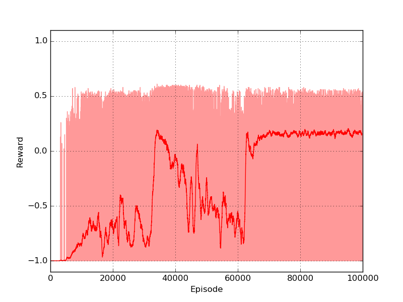
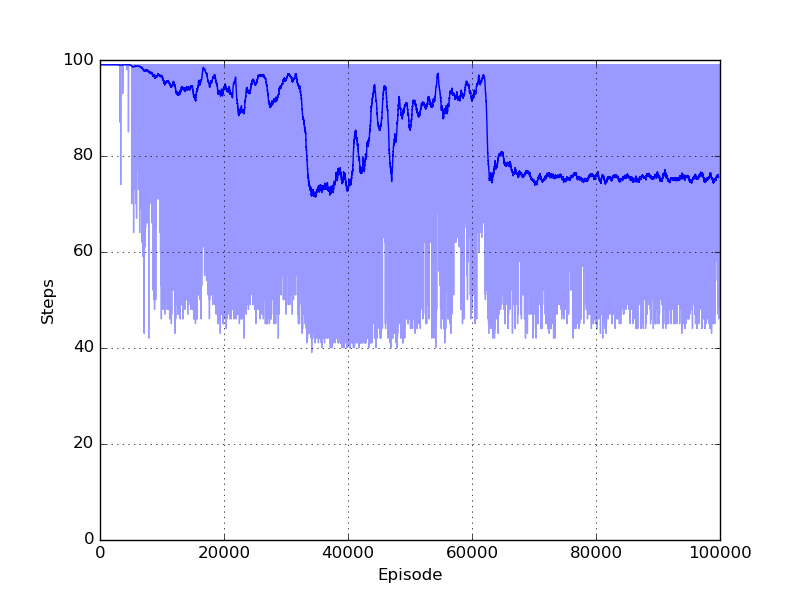
As it is possible to see a stable policy is obtained around episode \(65 \times 10^{3}\). At the same time a significant reduction in the number of steps necessary to finish the episode is showed in the step plot.

One of the policy that the algorithm obtained is very efficient and allows to reach the target position in 6.7 seconds with a cumulated reward of 0.34. The script prints on terminal the policy, which is represented by three actions-symbols (<=left, O=noop, >=right), the position (columns) and velocity (rows).

Episode: 100001
Epsilon: 0.1
Episode steps: 67
Cumulated Reward: 0.34
Policy matrix: 
 O   <   O   O   O   <   >   <   >   O   O   <
 <   <   >   <   <   >   <   <   >   >   O   >
 O   >   <   <   <   <   <   <   >   <   O   <
 O   <   <   <   >   >   <   <   >   >   <   O
 O   >   <   <   >   >   >   <   >   O   >   >
 O   >   >   <   >   O   >   <   >   >   <   <
 <   O   >   <   >   >   <   <   >   >   >   >
 O   >   <   <   >   >   >   >   >   >   >   >
 <   >   >   >   >   >   >   >   >   >   >   >
 O   >   >   >   >   >   >   >   >   >   O   >
 <   <   >   >   >   >   O   >   >   >   >   >
 >   O   >   >   >   >   >   >   >   <   >   <

The policy obtained is a sub-optimal policy. As it is possible to see from the step plot (light-blue curve) there are policies that can reach the goal in around 40 steps (4 seconds). The policy can be observed in the gif generated at the end of the training:

The discretization method worked well in the mountain car problem. However there are some possible issues that may occur. First of all, it is hard to decide how many bins one should use for the discretization. An high number of bins leads to a fine control but they can cause a combinatorial explosion. The second issue is that it may be necessary to visit all the states in order to obtain a good policy and this can lead to long training time. We will see in the rest of the series how to deal with these problems. For the moment you should download the complete code, which is called sarsa_mountain_car.py, from the official repository and play with it changing the hyper-parameters for obtaining a better performance.

Inverted Pendulum

The inverted pendulum is another classical problem, which is considered a benchmark in control theory. James Roberge was probably the first author to present a solution to the problem in his bachelor thesis back in 1960. The problem consists of a pole hinged on a cart which must be moved in order to keep the pole in vertical position. The inverted pendulum is well described in chapter 4.5.1 of Sugiyama’s book. Here I will use the same mathematical notation. The state space consists of the angle \(\phi \in [\frac{-\pi}{2}, \frac{\pi}{2}]\) (rad) (which is zero when the pole is perfectly vertical) and the angular velocity \(\dot{\phi} \in [-\pi, \pi]\) (rad/sec). The action space is discrete and it consists of three forces [-50, 0, 50] (Newton) which can be applied to the cart in order to swing the pole up.

The system has different parameters which can decide the dynamics. The mass \(m = 2 kg\) of the pole, the mass \(M = 8 kg\) of the cart, the lengh \(d = 0.5 m\) of the pole, and time step \(\Delta t = 0.1 s\). Given these parameters the angle \(\phi\) and the angular velocity \(\dot{\phi}\) at \(t+1\) are update as follows:

\[\phi_{t+1} = \phi_{t} + \dot{\phi}_{t+1} \Delta t\] \[\dot{\phi_{t+1}} = \dot{\phi_{t}} + \frac{g \ sin(\phi_t) - \alpha \ m \ d \ (\dot{\phi}_t)^2 \ sin(2\phi_t)/2 + \alpha \ cos(\phi_t) \ a_t }{ 4l/3 - \alpha \ m \ d \ cos^2(\phi_t)} \Delta t\]

Here \(\alpha = 1 / M+m\), and \(a_t\) is the action at time \(t\). The reward is updated considering the cosine of the angle \(\phi\), meaning larger the angle lower the reward. The reward is 0.0 when the pole is horizontal and 1.0 when vertical. When the pole is completely horizontal the episode finishes. Like in the mountain car example we can use discretization to enclose the continuous state space in pre-defined bins. For example, the position is codified with an angle in the range \([\frac{-\pi}{2}, \frac{\pi}{2}]\) and it can be discretized in 4 bins. When the pole has an angle of \(\frac{-\pi}{5}\) it is in the third bin, when it has an angle of \(\frac{\pi}{6}\) it is in the second bin, etc.

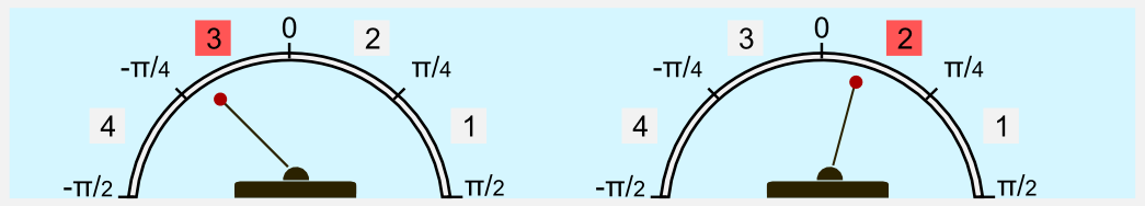
I wrote a special module called inverted_pendulum.py containing the class InvertedPendulum. Like in the mountain car module there are the methods reset(), step(), and render() which allow starting the episode, moving the pole and saving a gif. The animation is produced using Matplotlib and can be imagined as a camera centred on the cartpole main joint which moves in accordance with it. To create a new environment it is necessary to create a new instance of the InvertedPendulum object, defining the main parameters (masses, pole length and time step).

from inverted_pendulum import InvertedPendulum

# Defining a new environment with pre-defined parameters
my_pole = InvertedPendulum(pole_mass=2.0, 
                           cart_mass=8.0, 
                           pole_lenght=0.5, 
                           delta_t=0.1)

We can test the performance of an agent which follows a random policy. The code is called random_agent_inverted_pendulum.py and is available on the repository. Using a random strategy on the pole balancing environment leads to unsatisfactory performances. The best I got running the script multiple times is a very short episode of 1.5 seconds.

The optimal policy consists in compensating the angle and speed variations keeping the pole as much vertical as possible. Like for the mountain car I will deal with this problem using discretization. Both velocity and angle are discretized in bins of equal size and the resulting arrays are used as indices of a square policy matrix. As algorithm I will use first-visit Monte Carlo for control, which has been introduced in the second post of the series. I trained the policy for \(5 \times 10^5\) episodes (gamma=0.999, tot_bins=12). In order to encourage exploration I used an \(\epsilon\)-greedy strategy with \(\epsilon\) linearly decayed from 0.99 to 0.1. Each episode was 100 steps long (10 seconds). The maximum reward that can be obtained is 100 (the pole is kept perfectly vertical for all the steps). The reward plot shows that the algorithm could rapidly find good solutions, reaching an average score of 45.

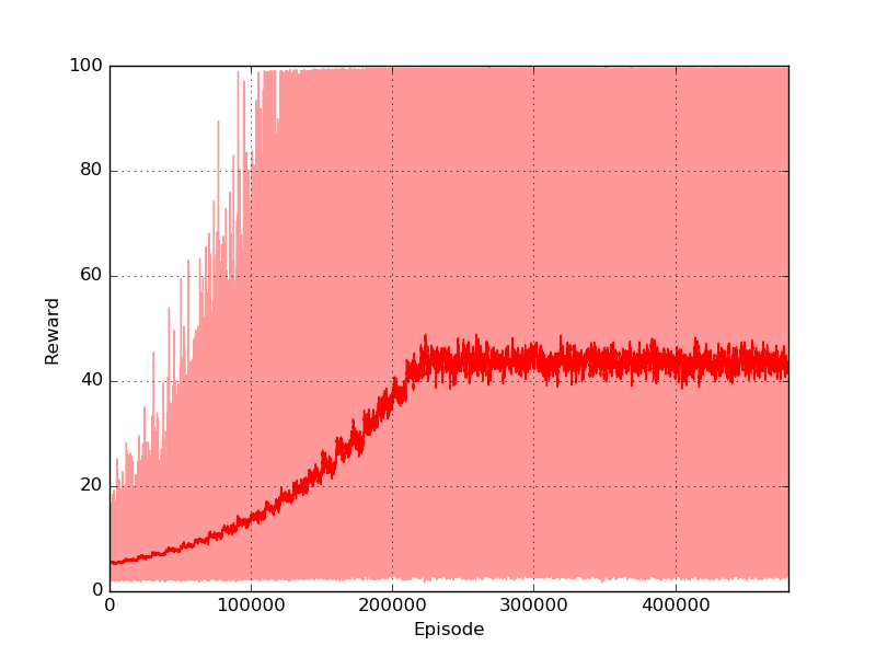
The final policy has a very good performance and with a favourable starting position can easily manage to keep the pole in balance for the whole episode (10 seconds).

The complete code is called montecarlo_control_inverted_pendulum.py and is included in the Github repository of the project. Feel free to change the parameters and check if they have an impact on the learning. Moreover you should test other algorithms on the pole balancing problem and verify which one gets the best performance.

Drone landing

There are plenty of possible applications for reinforcement learning. One of the most interesting is robots control. Reinforcement learning offers a wide set of techniques for the implementation of complex policies. For example, it has been applied to humanoid control, and helicopter acrobatic maneuvers. For a recent survey I suggest you to read the article of Kober et at. (2013). In this example we are going to use reinforcement learning for the control of an autonomous drone. In particular we have to train the drone to land on a ground platform.

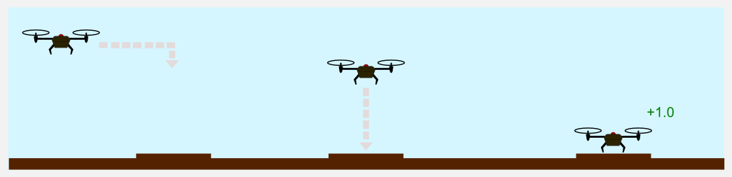
The drone moves in a discrete 3D world, represented by a cube. The marker is always in the same point (the centre of the floor). The rules are similar to the ones used in the gridworld. If the drone hits one of the wall it bounces back to the previous position. Landing on the platform leads to a positive reward of +1.0, while landing on another point leads to a negative reward of -1.0. A negative cost of living of -0.01 is applied at each time step. There are six possible actions: forward, backward, left, right, up, down. To simplify our lives we suppose that the environment is fully deterministic and that each action leads to a movement of 1 meter. This example is particularly useful to understand the combinatorial explosion and the effects on a reinforcement learning algorithm which is based on a simple lookup table.

I implemented a Python package called drone_lading.py which contains the class DroneLanding. Using this class it is possible to create a new environment in a few lines:

from drone_landing import DroneLanding

my_drone = DroneLanding(world_size=11)

The only requirement is the size of the world in meters. The class implements the usual methods step(), reset() and render(). The step method takes an integer representing one of the six actions (forward, backward, left, right, up, down) and returns the observation at t+1 represented by a tuple (x,y,z) which identifies the position of the drone. As usual the method returns also the reward and the boolean variable done which is True in case of a terminal state (the drone landed). The method render() is based on matplotlib and generates a gif or a video with the movement of the drone in a three-dimensional graph. Let’s start with a random agent, here is the code:

from drone_landing import DroneLanding
import numpy as np

my_drone = DroneLanding(world_size=11)
cumulated_reward = 0
print("Starting random agent...")
for step in range(50):
    action = np.random.randint(low=0, high=6)
    observation, reward, done = my_drone.step(action)
    print("Action: " + str(action))
    print("x-y-z: " + str(observation))
    print("")
    cumulated_reward += reward
    if done: break
print("Finished after: " + str(step+1) + " steps")
print("Cumulated Reward: " + str(cumulated_reward))
my_drone.render(file_path='./drone_landing.gif', mode='gif')
print("Complete!")

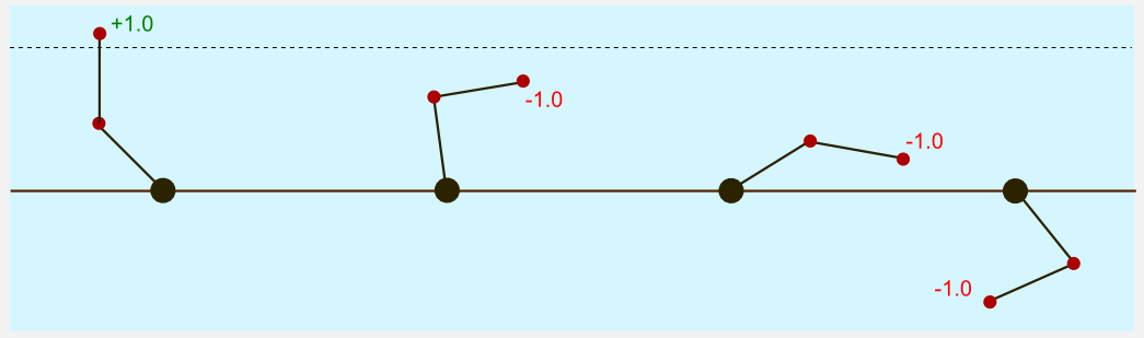
Running the script several times you can have an idea of how difficult is the task. It is very hard to reach the platform using a random strategy. In a world of size 11 meters, there is only 0.07% probability of obtaining the reward. Here you can see the gif generated for an episode of the random agent.

The drone is represented with a red dot, the red surface represents the area where landing leads to a negative reward, and the green square in the centre is the platform. As you can see the drone keeps moving in the same part of the room and complete the episode without landing at all. Here I will tackle the problem using Q-learning, a technique that has been introduced in the third post of the series. The code is pretty similar to the one used for the gridworld and you can find it in the official repository in the file called qlearning_drone_landing.py. The average cumulated reward for each episode (50 steps) is maximum 1.0 (if the drone land at the very first step), it is -1.5 if the drone is so unlucky to land outside of the platform at the very last step, and it is -0.5 if the drone keeps moving without landing at all (sum of the negative cost of living -0.01 for the 50 steps). Running the script for \(5 \times 10^{5}\) episodes, using an epsilon-greedy strategy (epsilon=0.1) I got the following result:

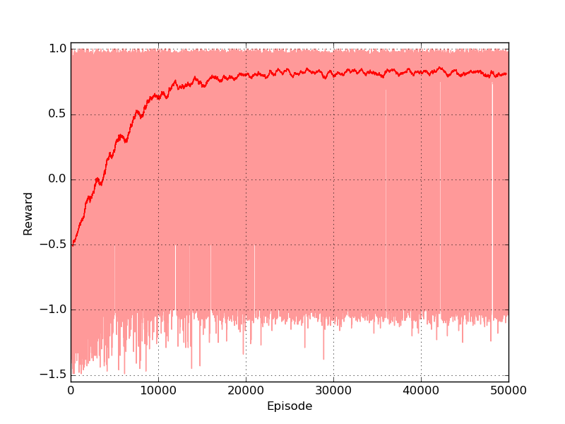
The algorithm converged pretty rapidly. The reward passed from negative (in the first 1000 episodes) to positive and it kept growing until reaching an average value of 0.9. The training took approximately 3 minutes on my laptop (Intel quad-core i5). Giving a look to the gif generated with the method render() we can see how the drone immediately moves toward the platform, reaching it in only 10 seconds.

Using a world of 11 meter was pretty easy to get a stable policy. Let’s try now with a world of 21 meters. In the script qlearning_drone_landing.py you simply have set the parameter world_size=21. In this new environment the probability of obtaining a reward goes down to 0.01%. I will not change any other parameter, because in this way we can compare the performance of the algorithm on this world with the performance on the previous one.

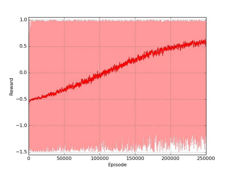
If you look to the plot you will notice two things. First, the reward grows extremely slowly, reaching an average of 0.6. Second, the number of episodes is much higher. I had to train the policy for \(25 \times 10^{5}\) episodes, four times more than in the previous environment. It took 40 minutes on the same laptop of the previous experiment. Giving a look to the gif created at the end of the training, we can see that eventually the policy is robust enough to guarantee the landing on the platform.

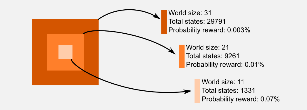
At this point it should be clear why using a lookup table for storing the state-action utilities is a limited approach. When the state-space grows we need to increase the size of the table. Starting from a world of size 11 and 6 total actions, we need a lookup table of size \(11 \times 11 \times 11 = 1331\) in order to store all the states, and a table of size \(11 \times 11 \times 11 \times 6 = 7986\) in order to store all the state-action pairs. Doubling the size of the world to 21 we have to increase the table of approximately 9 times. Moving to a world of size 31 we need a table which is 25 times larger. In the following image I summarized these observations. The orange squares represent the size of the lookup table required to store the state-action pairs, darker the square larger the table.

The problem related to explore a large dimensional space get worst and worst with the number of dimensions considered. In our case we had only three-dimensions to take into account, but considering larger hyper-spaces makes everything more complicated. This is a well known problem named curse of dimensionality, a term which has been coined by Richard Bellman (a guy that you should know, go to the first post to recall who is he). Only in the next post we will see how to overcome this problem using an approximator. In the last section I want to introduce other problems, problems which are considered extremely hard and that cannot be solved so easily.

Hard problems

The problem that I described above are difficult but not extremely difficult. In the end we managed to find good policies using a tabular approach. Which kind of problems are hard to solve using reinforcement learning?

An example is the acrobot. The acrobot is a planar robot represented by two links of equal length. The first link is connected to a fixed joint. The second link is connected to the first and both of them can swing freely and can pass by each other. The robot can control the torque applied to the second joint in order to swing and move the system. The state space is represented by the two positions of the links and by the two velocities. The action space is represented by the amount of torque the robot can apply to the joint. At the beginning of the episode the two links point downward. The goal is to swing the links until the tip passes a specific boundary. The reward given is negative (-1.0) until the robot reaches the terminal state (+1.0). The state space of the acrobot is large and it is challenging for our discrete approach. It is like having two inverted pendula which interact in the same system. Moreover the positive reward is sparse, meaning that it can be obtained only after a long series of coordinated movements. The acrobot is described in chapter 11.3 of the Sutton and Barto’s book. Sutton used SARSA(\(\lambda\)) and a linear approximator to solve the problem. We still do not have the right tools for mastering this problem, only in the next post we will see what a linear approximator is. If you are interested in the Sutton’s solution you can read this paper. Moreover if you want to try one of the algorithms on this problem you can use the implementation in OpenAI Gym. There is something harder than acrobot? Yes, an ensemble of acrobots: humanoid control.

A humanoid puppet has many degrees of freedom, and coordinating all of them is really hard. The state space is large and is represented by the velocity and position of multiple joints that must be controlled in synchrony in order to achieve an effective movement. The action space is the amount of torque it is possible to apply to each joint. Joint position, joint velocity and torque are continuous quantities. The reward function depends on the task. For example, in a bipedal walker the reward could be the distance reached by the puppet in a finite amount of time. Trying to obtain decent results using a discretised approach is infeasible. During the years different techniques have been applied with more or less success. Despite recent advancement humanoid control is still considered an open problem. If you want to try there is an implementation of a bipedal walker in OpenAI Gym. There is something harder than humanoid control? Probably yes, what about videogames?

If you played with the 2600 Atari games you may have noticed that some of them are really hard. How can an algorithm play those games? Well, we can cheat. If the game can be reduced to a limited set of features, it is possible to use model based reinforcement learning to solve it. However most of the time the reward function and the transition matrix are unknown. In these cases the only solution is to use the raw coulour image as state space. The state space represented by a raw image is extremely large. There is no point in using a lookup table for such a big space because most of the states will remain unvisited. We should use an approximator which can describe with a reduced set of parameters the state space. Soon I will show you how deep reinforcement learning can use neural networks to master this kind of problems.

Conclusions

Here I presented some classical reinforcement learning problems showing how the techniques of the previous posts can be used to obtain stable policies. However we always started from the assumption of a discretized state space which was described by a lookup table or matrix. The main limitation of this approach is that in many applications the state space is extremely large and it is not possible to visit all the states. To solve this problem we can use function approximation. In the next post I will introduce function approximation and I will show you how a neural network can be used in order to describe a large state space. The use of neural networks open up new horizons and it is the first step toward modern methods such as deep reinforcement learning.

Index

1. [First Post] Markov Decision Process, Bellman Equation, Value iteration and Policy Iteration algorithms.
2. [Second Post] Monte Carlo Intuition, Monte Carlo methods, Prediction and Control, Generalised Policy Iteration, Q-function.
3. [Third Post] Temporal Differencing intuition, Animal Learning, TD(0), TD(λ) and Eligibility Traces, SARSA, Q-learning.
4. [Fourth Post] Neurobiology behind Actor-Critic methods, computational Actor-Critic methods, Actor-only and Critic-only methods.
5. [Fifth Post] Evolutionary Algorithms introduction, Genetic Algorithm in Reinforcement Learning, Genetic Algorithms for policy selection.
6. [Sixt Post] Reinforcement learning applications, Multi-Armed Bandit, Mountain Car, Inverted Pendulum, Drone landing, Hard problems.
7. [Seventh Post] Function approximation, Intuition, Linear approximator, Applications, High-order approximators.
8. [Eighth Post] Non-linear function approximation, Perceptron, Multi Layer Perceptron, Applications, Policy Gradient.

Resources

• The complete code for the Reinforcement Learning applications is available on the dissecting-reinforcement-learning official repository on GitHub.

• Reinforcement learning: An introduction (Chapter 11 ‘Case Studies’) Sutton, R. S., & Barto, A. G. (1998). Cambridge: MIT press. [html]

• History of Inverted-Pendulum Systems Lundberg, K. H., & Barton, T. W. (2010). [pdf]

• Reinforcement Learning on autonomous humanoid robots Schuitema, E. (2012). [pdf]

• Generalization in reinforcement learning: Successful examples using sparse coarse coding Sutton, R. S. (1996). [pdf]

References

Abbeel, P., Coates, A., Quigley, M., & Ng, A. Y. (2007). An application of reinforcement learning to aerobatic helicopter flight. In Advances in neural information processing systems (pp. 1-8).

Kober, J., Bagnell, J. A., & Peters, J. (2013). Reinforcement learning in robotics: A survey. The International Journal of Robotics Research, 32(11), 1238-1274.

Lundberg, K. H., & Barton, T. W. (2010). History of inverted-pendulum systems. IFAC Proceedings Volumes, 42(24), 131-135.

Sutton, R. S. (1996). Generalization in reinforcement learning: Successful examples using sparse coarse coding. In Advances in neural information processing systems (pp. 1038-1044).

Thompson, W. R. (1933). On the likelihood that one unknown probability exceeds another in view of the evidence of two samples. Biometrika, 25(3/4), 285-294.