Dissecting Reinforcement Learning-Part.4

Here we are, the fourth episode of the “Dissecting Reinforcement Learning” series. In this post I will introduce another group of techniques widely used in reinforcement learning: Actor-Critic (AC) methods. I often define AC as a meta-technique that uses the methods introduced in the previous posts in order to learn. AC-based algorithms are among the most popular methods in reinforcement learning. For example, the Deep Determinist Policy Gradient algorithm introduced recently by some researchers at Google DeepMind is an actor-critic, model-free method. Moreover, the AC framework has many connections with neuroscience and animal learning, in particular with models of basal ganglia (Takahashi et al. 2008).

AC methods are not accurately described in the books I generally provide. For instance in Russel and Norvig and in the Mitchell’s book they are not covered at all. In the classical Sutton and Barto’s book there are only three short paragraphs (2.8, 6.6, 7.7), however in the second edition a wider description of neuronal AC methods has been added in chapter 15 (neuroscience). A meta-classification of reinforcement learning techniques is covered in the article “Reinforcement Learning in a Nutshell”. Here, I will introduce AC methods starting from neuroscience. You can consider this post as the neuro-physiological counterpart of the third one, that introduced Temporal Differencing (TD) methods from a psychological and behaviouristic point of view.

Actor-Critic methods (and rats)

AC methods are deeply connected with neuroscience, therefore I will introduce this topic with a brief excursion in the neuroscience field. If you have a pure computational background you will learn something new. My objective is to give you a deeper insight into the reinforcement learning (extended) world. To understand this introduction you should be familiar with the basic structure of the nervous system. What is a neuron? How do neurons communicate using synapses and neurotransmitters? What is the cerebral cortex? You do not need to know the details, here I want you to get the general scheme. Let’s start from Dopamine. Dopamine is a neuromodulator implied in some of the most important process in human and animal brains. You can see dopamine as a messenger that allows neurons to communicate. Dopamine has an important role in multiple processes in the mammalian brain (e.g. learning, motivation, addiction), and it is produced in two specific areas: substantia nigra pars compacta and ventral tegmental area. These two areas have direct projections to another area of the brain, the striatum. The striatum is divided in two parts: ventral striatum and dorsal striatum. The output of the striatum is directed to motor areas and prefrontal cortex, and it is involved in motor control and planning.

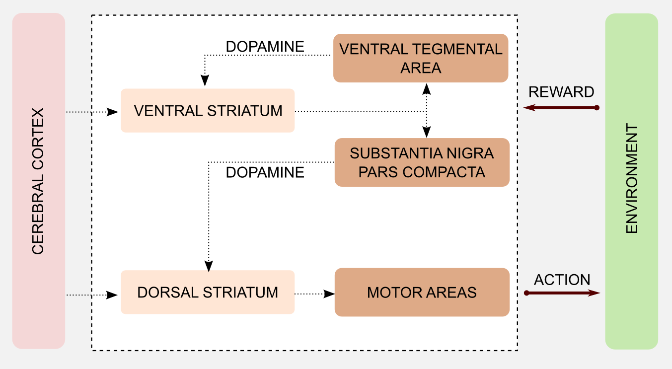
Most of the brain areas cited so far are part of the basal ganglia. Different models found a connection between basal ganglia and learning. In particular, it seems that the phasic activity of the dopaminergic neurons can encode an error. This error is very similar to the error in TD learning that I introduced in the third post. Before going into details I would like to simplify the basal ganglia mechanism distinguishing between two groups:

1. Ventral striatum, substantia nigra, ventral tegmental area
2. Dorsal striatum and motor areas

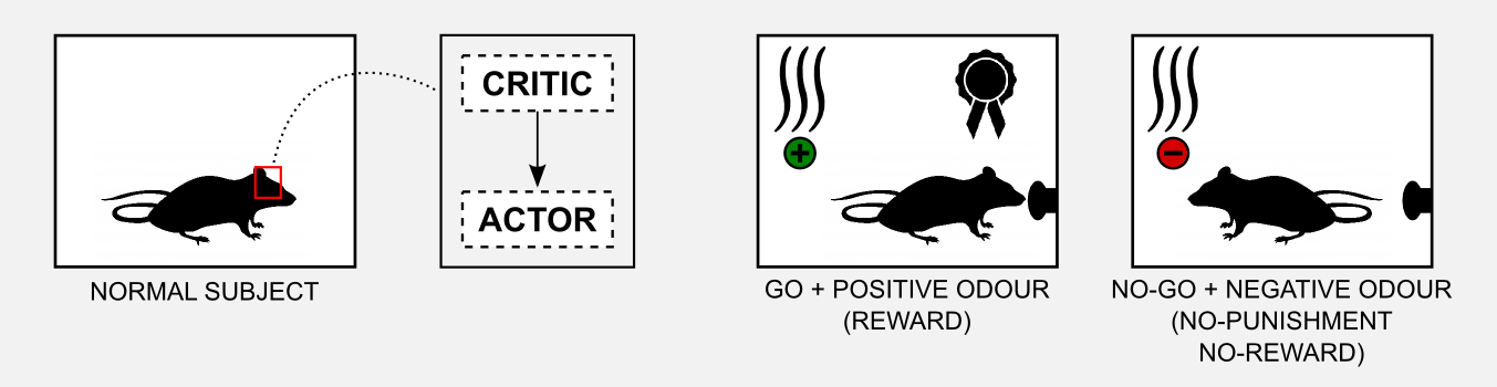
There are no specific biological names for these groups but I will create two labels for the occasion. The first group can evaluate the saliency of a stimulus based on the associated reward. At the same time it can estimate an error measure comparing the result of the action and the direct consequences, and use this value to calibrate an executor. For these reasons I will call it the critic. The second group has direct access to actions but no way to estimate the utility of a stimulus, because of that I will call it the actor.

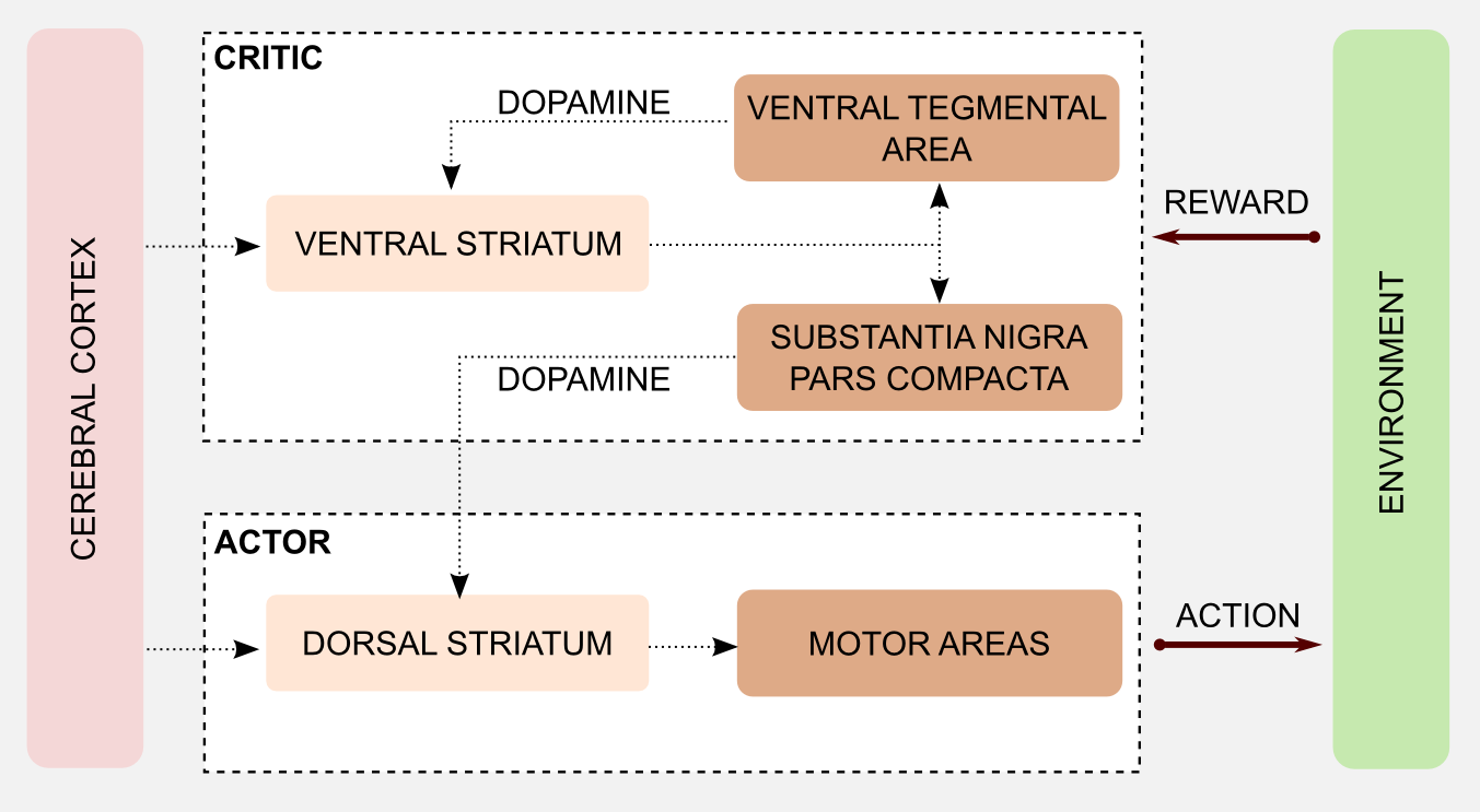
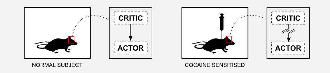
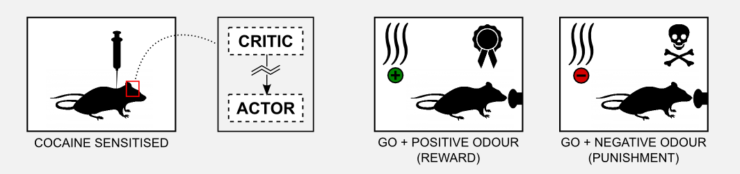
The interaction between actor and critic has an important role in learning. In particular, well established research has shown that basal ganglia are involved in Pavlovian learning (see third post) and in procedural (implicit) memory, meaning unconscious memories such as skills and habits. On the other hand the acquisition of declarative (explicit) memory, implied in the recollection of factual information, seems to be connected with another brain area called hippocampus. The only way actor and critic can communicate is through the dopamine released from the substantia nigra after the activation of the ventral striatum. Drug abuse can have an effect on the dopaminergic system, altering the communication between actor and critic. Some experiments of Takahashi et al. (2007) showed that cocaine sensitization in rats can have as effect maladaptive decision-making. In particular, rather than being influenced by long-term goal, rats are driven by immediate rewards. This issue is also part of standard computational pipelines and is know as the credit assignment problem. For example, when playing chess it is not easy to isolate the most salient actions that lead to the final victory (or defeat).

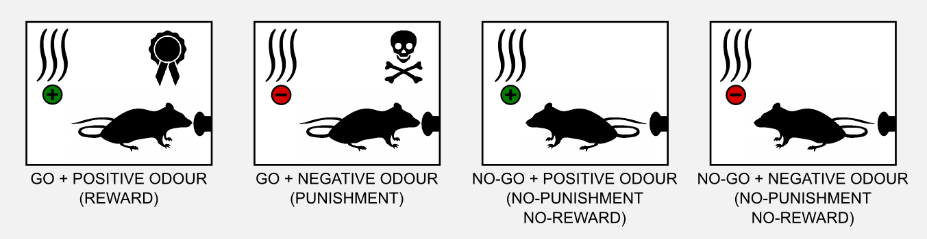
To understand how the neuronal actor-critic mechanism was involved in the credit assignment problem, Takahashi et al. (2008) observed the performances of rats pre-sensitized with cocaine in a Go/No-Go task. The procedure of a Go/No-Go task is simple. The rat is in a small metallic box and it has to learn to poke a button with the nose when a specific odour (cue) is released. If the rat pokes the button when a positive odour is present it gets rewarded (with delicious sugar). If the rat pokes the button when a negative odour is present it gets punished (e.g. with a bitter substance such as quinine). Positive and negative odours do not mean that they are pleasant or unpleasant, we can consider them neutral. Learning means to associate a specific odour to reward or punishment. Finally, if the rat does not move (No-Go) then neither reward nor punishment are given. In total there are four possible conditions.

The interesting fact observed in those experiments is that rats pre-sensitized with cocaine do not learn the task. The most plausible explanation is that cocaine damages the basal ganglia and the signal returned by the critic gets distorted. To test this hypothesis Takahashi et al. (2008) sensitized a group of rats 1-3 months before the experiment and then compared it with a non-sensitized control group. The results of the experiment showed that the rat in the control group could learn how to obtain the reward (go) when the positive odour was presented and how to avoid the punishment (no-go) when the negative odour was presented. The observations of the basal ganglia showed that the ventral striatum (critic) developed some cue-selectivity neurons that fired only when the odour appeared. This neurons developed during the training and their activity preceded the response in the dorsal striatum (actor).

On the other hand the cocaine sensitized rat did not show any kind of cue-selectivity during the training. Moreover, post-mortem analysis showed that those rats did not developed cue-selective neurons in the ventral striatum (critic). These results confirm the hypothesis that the critic learns the value of the cue and it instructs the actor about the action to execute.

In this section, I showed how the AC framework is deeply connected to the neurobiology of the mammalian brain. The model is elegant and it can explain phenomena such as Pavlovian learning and drug addiction. However, the elegance of the model does not have to prevent us from criticizing it. Be aware that there are different experiments that did not confirm it. For example, some form of stimulus-reward learning can take place in the absence of dopamine. Moreover dopamine cells can fire before the stimulus, meaning that their values cannot be used for the update. For a good review of neuronal AC models and their limits I suggest you the article of Joel et al. (2002).

Now it’s time to turn our attention to math and code. How can we build a computational model from the biological one?

Rewiring Actor-Critic methods

In the last section I presented a neuronal model of the basal ganglia based on the AC framework. Here, I will rewire that model using the reinforcement learning techniques we studied until now. The objective is to obtain a computational version which can be used in generic cases (e.g. the 4x3 grid world). The first implementation of an AC algorithm is due to Witten (1977), however the terms Actor and Critic have been introduced later by Barto et al. (1988) to solve the pole-balancing problem. First of all, how can we represent the critic? In the neural version the critic does not have access to the actions. Input to the critic is the information obtained through the cerebral cortex that we can compare to the information obtained by the agent through the sensors (state estimation). Moreover the critic receives as input a reward, this comes directly from the environment. The critic can be represented by an utility function, that is updated based on the reward signal received at each iteration. In model free reinforcement learning we can use the TD(0) algorithm to represent the critic. The dopaminergic output from substantia nigra and ventral tegmental area can be represented by the two signals returned by TD(0): the update value and the error estimation \(\delta\). In practice we use the update signal to improve the utility function and the error to update the actor. How can we represent the actor? In the neural system the actor receives an input from the cerebral cortex, that we can translate in sensor signals (current state). The dorsal striatum projects to the motor areas and executes an action. Similarly, we can use a state-action matrix containing the possible actions for each state. The action can be selected with an ε-greedy (or softmax) strategy and then updated using the error returned by the critic. As usual a picture is worth a thousand words:

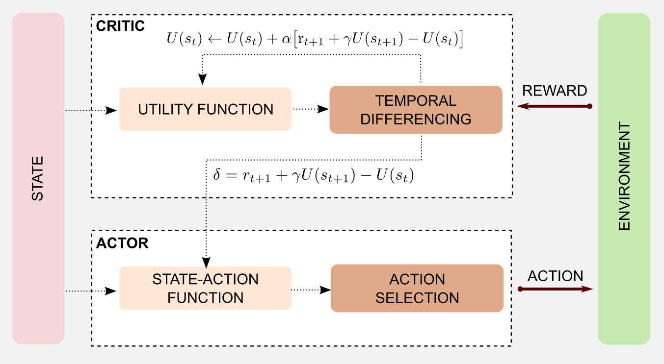
We can summarize the steps of the AC algorithm as follows:

1. Produce the action \(a_{t}\) for the current state \(s_{t}\)
2. Observe next state \(s_{t+1}\) and the reward \(r\)
3. Update the utility of state \(s_{t}\) (critic)
4. Update the probability of the action using \(\delta\) (actor)

In step 1, the agent produces an action following the current policy. In the previous posts I used an ε-greedy strategy to select the action and to update the policy. Here, I will select a certain action using a softmax function:

\[P \big\{ a_{t}=a | s_{t}=s \big\} = \frac{e^{p(s,a)}}{\sum_{b} e^{p(s,b)}}\]

After the action we observe the new state and the reward (step 2). In step 3 we plug the reward, the utility of \(s_{t}\) and \(s_{t+1}\) in the standard update rule used in TD(0) (see third post):

\[U(s_{t}) \leftarrow U(s_{t}) + \alpha \big[ \text{r}_{t+1} + \gamma U(s_{t+1}) - U(s_{t}) \big]\]

In step 4 we use the error estimation \(\delta\) to update the policy. In practical terms, step 4 consists of strengthening or weakening the probability of the action using the error \(\delta\) and a positive step-size parameter \(\beta\):

\[p(s_{t}, a_{t}) \leftarrow p(s_{t}, a_{t}) + \beta \delta_{t}\]

Like in the TD case, we can also integrate the eligibility traces mechanism (see third post). In the AC case we need two set of traces, one for the actor and one for the critic. For the critic we need to store a trace for each state and update it as follows:

\[e_{t}(s) = \begin{cases} \gamma \lambda e_{t-1}(s) & \text{if}\ s \neq s_{t}; \\ \gamma \lambda e_{t-1}(s)+1 & \text{if}\ s=s_{t}; \end{cases}\]

Nothing different from the TD(λ) method I introduced in the third post. Once we estimated the trace we can update the state as follows:

\[U(s_{t}) \leftarrow U(s_{t}) + \alpha \delta_{t} e_{t}(s)\]

For the actor we have to store a trace for each state-action pair, similarly to SARSA and Q-learning. The traces can be updated as follows:

\[e_{t}(s,a) = \begin{cases} \gamma \lambda e_{t-1}(s,a)+1 & \text{if}\ s=s_{t} \text{ and } a=a_{t}; \\ \gamma \lambda e_{t-1}(s,a) & \text{otherwise}; \end{cases}\]

Finally, the probability of choosing an action is updated as follows:

\[p(s_{t}, a_{t}) \leftarrow p(s_{t}, a_{t}) + \alpha \delta_{t} e_{t}(s)\]

Great, we obtained our generic computational model to use in a standard reinforcement learning scenario. Now, I would like to close the loop providing an answer to this simple question: does the computational model explain the neurobiological observation? Apparently yes. In the previous section we saw how Takahashi et al. (2008) observed some anomalies in the interaction between actor and critic in rats sensitized with cocaine. Drug abuse seems to deteriorate the dopaminergic feedback going from the critic to the actor. From the computational point of view we can observe a similar result when all the \(U(s)\) are the same regardless of the current state. In this case the prediction error \(\delta\) generated by the critic (with \(\gamma=1\)) reduces to the immediate available reward:

\[\delta_{t} = r_{t+1} + U(s_{t+1}) - U(s_{t}) = r_{t+1}\]

This result explains why the credit assignment problem emerges during the training of cocaine sensitized rats. The rats prefer the immediate reward and do not take into account the long-term drawbacks. Learning based only on immediate reward it’s not sufficient to master a complex Go/No-Go task but in simpler tasks learning can be faster, with cocaine sensitized rats performing better than the control group. However, for a neuroscientist this sort of explanations are too tidy. Recent work has highlighted the existence of multiple learning systems operating in parallel in the mammalian brain. Some of these systems (e.g. amygdala and/or nucleus accumbens) can replace a malfunctioning critic and compensate the damage caused by cocaine sensitization. In conclusion, additional experiments are needed in order to shed light on the neuronal AC architecture. Now it is time for coding. In the next section I will show you how to implement an AC algorithm in Python and how to apply it to the cleaning robot example.

Actor-Critic Python implementation

Using the knowledge acquired in the previous posts we can easily create a Python script to implement an AC algorithm. As usual, I will use the robot cleaning example and the 4x3 grid world. To understand this example you have to read the rules of the grid world introduced in the first post. First of all I will describe the general architecture, then I will describe step-by-step the algorithm in a single episode. Finally I will implement everything in Python. In the complete architecture we can represent the critic using a utility function (state matrix). The matrix is initialized with zeros and updated at each iteration through TD learning. For example, after the first step the robot moves from (1,1) to (1,2) obtaining a reward of -0.04. The actor is represented by a state-action matrix similar to the one used to model the Q-function. Each time a new state is observed an action is returned and the robot moves. To avoid clutter I will draw an empty state-action matrix, but imagine that the values inside the table have been initialized with random samples in the range [0,1].

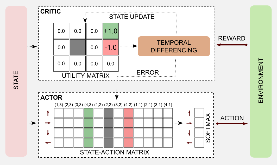
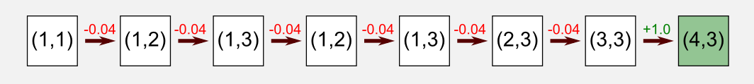
In the episode considered here the robot starts in the bottom-left corner at state (1,1) and it reaches the charging station (reward=+1.0) after seven steps.

The first thing to do is to take an action. A query to the state-action table (actor) returns the action vector for the current state that in our case is [0.48, 0.08, 0.15, 0.37]. The action vector is passed to the softmax function that turns it into a probability distribution [0.30, 0.20, 0.22, 0.27]. I sampled from the distribution using the Numpy method np.random.choice() that returned the action UP.

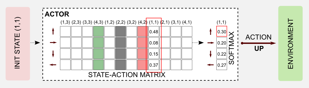
The softmax function took as input the N-dimensional action vector \(\boldsymbol{x}\) and returned an N-dimensional vector of real values in the range [0, 1] that add up to 1. The softmax function can be easily implemented in Python, however differently from the original softmax equation here I will use numpy.max() in the exponents to avoid approximation errors:

def softmax(x):
    '''Compute softmax values of array x.

    @param x the input array
    @return the softmax array
    '''
    return np.exp(x - np.max(x)) / np.sum(np.exp(x - np.max(x)))

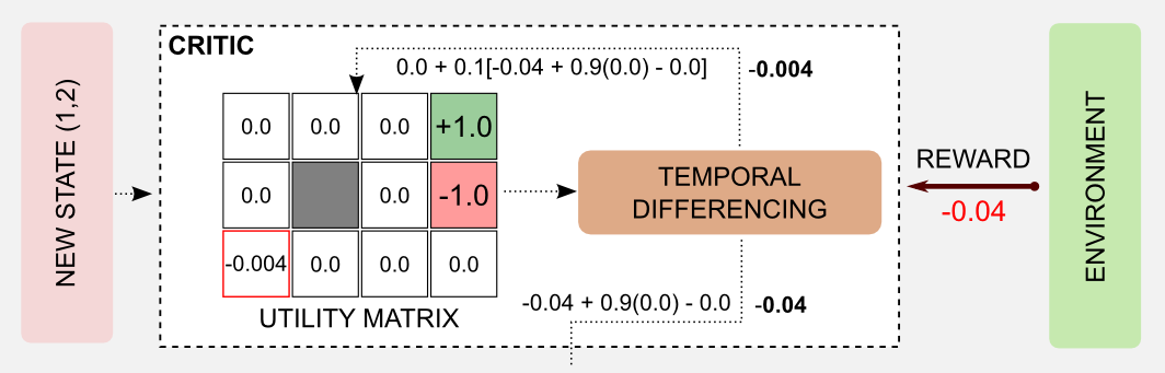
After the action, a new state is reached and a reward is available (-0.04). It’s time to update the state value of the critic and to estimate the error \(\delta\). Here, I used the following parameters: \(\alpha=0.1\), \(\beta=1.0\) and \(\gamma=0.9\). Applying the update rule (step 3 of the algorithm) we obtain the new value for the state (1,1): 0.0 + 0.1[-0.04 + 0.9(0.0) - 0.0] = -0.004. At the same time it is possible to calculate the error \(\delta\) as follows: -0.04 + 0.9(0.0) - 0.0 = -0.04

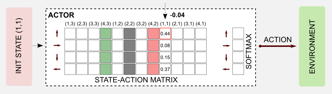
The robot is in a new state, and the the error has been evaluated by the critic. Now the error has to be used to update the state-action table of the actor. In this step, the action UP for state (1,1) is weakened, adding the negative term \(\delta\). In case of a positive \(\delta\) the action would be strengthened.

We can repeat the same steps until the end of the episode. All the action will be weakened but the last one, that will be strengthened by a factor of +1.0. Repeating the process for many episodes we get the optimal utility matrix and the optimal policy.

Time for the Python implementation. First of all, we have to create a function to update the utility matrix (critic). I called this function update_critic. The inputs are the utility_matrix, the observation and new_observation states, then the usual hyper-parameters. The function returns an updated utility matrix and the estimation error delta to use for updating the actor.

def update_critic(utility_matrix, observation, new_observation, 
                   reward, alpha, gamma):
    '''Return the updated utility matrix

    @param utility_matrix the matrix before the update
    @param observation the state obsrved at t
    @param new_observation the state observed at t+1
    @param reward the reward observed after the action
    @param alpha the ste size (learning rate)
    @param gamma the discount factor
    @return the updated utility matrix
    @return the estimation error delta
    '''
    u = utility_matrix[observation[0], observation[1]]
    u_t1 = utility_matrix[new_observation[0], new_observation[1]]
    delta = reward + gamma * u_t1 - u
    utility_matrix[observation[0], observation[1]] += alpha * (delta)
    return utility_matrix, delta

The function update_actor is used to update the state-action matrix. The parameter passed to the function are the state_action_matrix, the observation, the action, the estimation error delta (returned by update_critic), and the hyper-parameter beta (represented as a matrix with a value for each pair) counting how many times a particular state-action pair has been visited.

def update_actor(state_action_matrix, observation, action, 
                 delta, beta_matrix=None):
    '''Return the updated state-action matrix

    @param state_action_matrix the matrix before the update
    @param observation the state obsrved at t
    @param action taken at time t
    @param delta the estimation error returned by the critic
    @param beta_matrix a visit counter for each state-action pair
    @return the updated matrix
    '''
    col = observation[1] + (observation[0]*4)
    if beta_matrix is None: beta = 1
    else: beta = 1 / beta_matrix[action,col]
    state_action_matrix[action, col] += beta * delta
    return state_action_matrix 

The two functions are used in the main loop. The exploring start assumption is once again used here to guarantee uniform exploration. The beta_matrix parameter has not been used in this example, but it can be easily enabled.

for epoch in range(tot_epoch):
  #Reset and return the first observation
  observation = env.reset(exploring_starts=True)
  for step in range(1000):
    #Estimating the action through Softmax
    col = observation[1] + (observation[0]*4)
    action_array = state_action_matrix[:, col]
    action_distribution = softmax(action_array)
    #Sampling an action using the probability
    #distribution returned by softmax
    action = np.random.choice(4, 1, p=action_distribution)
    #beta_matrix[action,col] += 1 #increment the counter
    #Move one step in the environment and get obs and reward
    new_observation, reward, done = env.step(action)
    #Updating the critic (utility_matrix) and getting the delta
    utility_matrix, delta = update_critic(utility_matrix, observation, 
                                          new_observation, reward, 
                                          alpha, gamma)
    #Updating the actor (state-action matrix)
    state_action_matrix = update_actor(state_action_matrix, observation, 
                                       action, delta, beta_matrix=None)
    observation = new_observation
    if done: break

I uploaded the complete code in the official GitHub repository under the name actor_critic.py. Running the script with gamma = 0.999 and alpha = 0.001 I obtained the following utility matrix:

Utility matrix after 1001 iterations:
[[-0.02564938  0.07991029  0.53160489  0.        ]
 [-0.054659    0.          0.0329912   0.        ]
 [-0.06327405 -0.06371056 -0.0498283  -0.11859039]]

...

Utility matrix after 150001 iterations:
[[ 0.85010645  0.9017371   0.95437213  0.        ]
 [ 0.80030524  0.          0.68354459  0.        ]
 [ 0.72840853  0.55952242  0.60486472  0.39014426]]

...

Utility matrix after 300000 iterations:
[[ 0.84762914  0.90564964  0.95700181  0.        ]
 [ 0.79807688  0.          0.69751386  0.        ]
 [ 0.72844679  0.55459785  0.60332219  0.38933992]]

Comparing the result obtained with AC and the one obtained with dynamic programming in the first post we can notice a few differences.

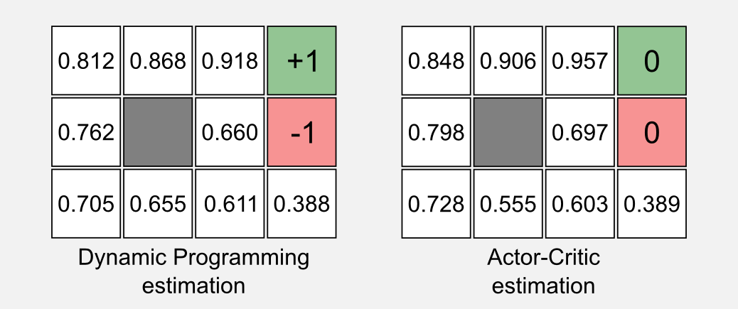
Similarly to the estimation of TD(0) in the third post the value of the two terminal states is zero. This is the consequence of the fact that we cannot estimate the update value for a terminal state, because after a terminal state there is no other state. As discussed in the third post this is not a big issue since it does not affect the convergence, and can be addressed with a simple conditional statement. From a practical point of view the results obtained with the AC algorithm can be unstable because there are more hyper-parameter to tune, however the flexibility of the paradigm can often balance this drawback.

Actor-only and Critic-only methods

In the Sutton and Barto’s book AC methods are considered part of TD methods. That makes sense, because the critic is an implementation of the TD(0) algorithm and it is updated following the same rule. The question is: why should we use AC methods instead of TD learning? The main advantage of AC methods is that the \(\delta\) returned by the critic is an error value produced by an external supervisor. We can use this value to adjust the policy with supervised learning. The use of an external supervisor reduces the variance when compared to pure Actor-only methods. These aspects will be clearer when I will introduce function approximators later on in the series. Another advantage of AC methods is that the action selection requires minimal computation. Until now we always had a discrete number of possible actions. When the action space is continuous and the possible number of action infinite, it is computationally prohibitive to search for the optimal action in this infinite set. AC methods can represent the policy in a separate discrete structure and use it to find the best action. Another advantage of AC methods is their similarity to the brain mechanisms of reward in the mammalian brain. This similarity makes AC methods appealing as psychological and biological models. To summarize there are three advantages in using AC methods:

1. Variance reduction in function approximation.
2. Computationally efficiency in continuous action space.
3. Similarity to biological reward mechanisms in the mammalian brain.

The distinction between actor and critic is also very useful from a taxonomic point of view. In the article “Reinforcement Learning in a Nutshell” AC methods are considered as a meta-category that can be used to assign all the techniques I introduced until now to three macro-groups: AC methods, Critic-only, Actor-only. Here I will follow a similar approach to give a wider view on what is available out there. In this post I introduced a possible architecture for an AC algorithm. In AC methods the actor and the critic are represented explicitly and trained separately, but we could ask: is it possible to use only the actor or only the critic? In previous posts we considered utility functions and policies. In dynamic programming these two entities collapsed in the value iteration and the policy iteration algorithms (see first post). Both those algorithms are based on utility estimation, that allows the policy to converge thanks to the Generalised Policy Iteration (GPI) mechanism (see second post). Note that, even in TD learning we are relying on utility estimation (see third post) especially when the emphasis is on the policy (SARSA and Q-learning). All these methods can be broadly grouped in a category called Critic-only. Critic-only methods always build a policy on top of a utility function and as I said the utility function is the critic in the AC framework.

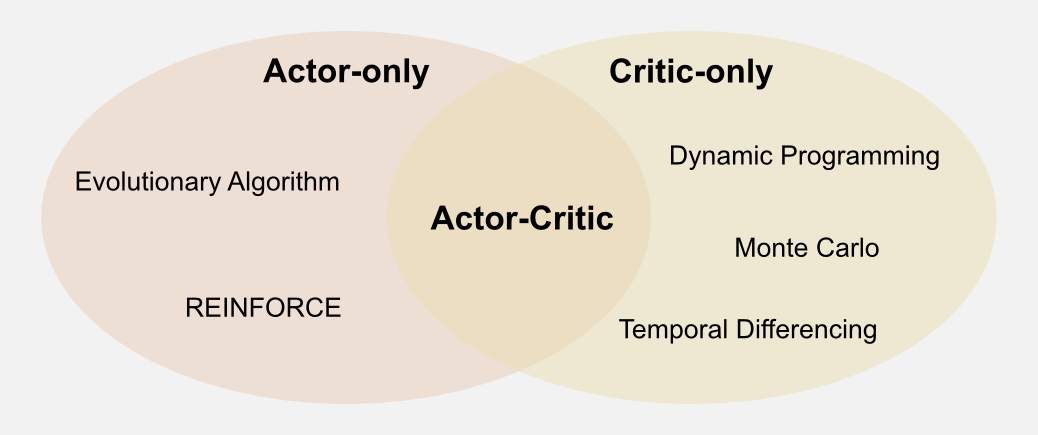
What if we search for an optimal policy without using a utility function? Is that possible? The answer is yes. We can search directly in policy space using an Actor-only approach. A class of algorithms called REINFORCE (REward Increment = Nonnegative Factor x Offset Reinforcement x Characteristic Eligibility) can be considered part of the Actor-only group. REINFORCE measures the correlation between the local behaviour and the global performance of the agent and updates the weights of a neural network. To understand REINFORCE it is necessary to know gradient descent and generalisation through neural networks (which I will cover later in this series). Here, I would like to focus more on another type of Actor-only techniques: evolutionary algorithms. The evolutionary algorithm label can be applied to a wide range of techniques, but in reinforcement learning are often used genetic algorithms. Genetic algorithms represent each policy as a possible solution to the agent problem. Imagine 10 cleaning robots working in parallel, each one using a different (random initialized policy). After 100 episodes we can have an estimation of how good the policy of each single robot is. We can keep the best robots and randomly mutate their policies in order to generate new ones. After some generations, evolution selects the best policies and among them we can (probably) find the optimal one. In classic reinforcement learning textbooks the genetic algorithms are not covered, but I had first-hand experience with them. When I was an undergraduate I did an internship at the Laboratory of Autonomous Robotics and Artificial Life (LARAL), where I used genetic algorithms in evolutionary robotics to investigate the decision making strategies of simulated robots living in different ecologies. I will spend more words on genetic algorithms for reinforcement learning in the next post.

Conclusions

Starting from the neurobiology of the mammalian brain I introduced AC methods, a class of reinforcement learning algorithms widely used by the research community. The neuronal AC model can describe phenomena like Pavlovian learning and drug addiction, whereas its computational counterpart can be easily applied to robotics and machine learning. The Python implementation is straightforward and is based on the TD(0) algorithm introduced in the third post. AC methods are also good for taxonomic reasons, we can categorize TD algorithms as Critic-only methods and techniques such as REINFORCE and genetic algorithm as Actor-only methods. In the next post I will focus on genetic algorithms, a method that allows us to search directly in the policy space without the need of a utility function.

Index

1. [First Post] Markov Decision Process, Bellman Equation, Value iteration and Policy Iteration algorithms.
2. [Second Post] Monte Carlo Intuition, Monte Carlo methods, Prediction and Control, Generalised Policy Iteration, Q-function.
3. [Third Post] Temporal Differencing intuition, Animal Learning, TD(0), TD(λ) and Eligibility Traces, SARSA, Q-learning.
4. [Fourth Post] Neurobiology behind Actor-Critic methods, computational Actor-Critic methods, Actor-only and Critic-only methods.
5. [Fifth Post] Evolutionary Algorithms introduction, Genetic Algorithms in Reinforcement Learning, Genetic Algorithms for policy selection.
6. [Sixt Post] Reinforcement learning applications, Multi-Armed Bandit, Mountain Car, Inverted Pendulum, Drone landing, Hard problems.
7. [Seventh Post] Function approximation, Intuition, Linear approximator, Applications, High-order approximators.
8. [Eighth Post] Non-linear function approximation, Perceptron, Multi Layer Perceptron, Applications, Policy Gradient.

Resources

• The complete code for the Actor-Critic examples is available on the dissecting-reinforcement-learning official repository on GitHub.

• Reinforcement learning: An introduction. Sutton, R. S., & Barto, A. G. (1998). Cambridge: MIT press. [html]

• Reinforcement learning: An introduction (second edition). Sutton, R. S., & Barto, A. G. (in progress). [pdf]

• Reinforcement Learning in a Nutshell. Heidrich-Meisner, V., Lauer, M., Igel, C., & Riedmiller, M. A. (2007) [pdf]

References

Barto, A. G., Sutton, R. S., & Anderson, C. W. (1983). Neuronlike adaptive elements that can solve difficult learning control problems. IEEE transactions on systems, man, and cybernetics, (5), 834-846.

Heidrich-Meisner, V., Lauer, M., Igel, C., & Riedmiller, M. A. (2007, April). Reinforcement learning in a nutshell. In ESANN (pp. 277-288).

Joel, D., Niv, Y., & Ruppin, E. (2002). Actor–critic models of the basal ganglia: New anatomical and computational perspectives. Neural networks, 15(4), 535-547.

Takahashi, Y., Roesch, M. R., Stalnaker, T. A., & Schoenbaum, G. (2007). Cocaine exposure shifts the balance of associative encoding from ventral to dorsolateral striatum. Frontiers in integrative neuroscience, 1(11).

Takahashi, Y., Schoenbaum, G., & Niv, Y. (2008). Silencing the critics: understanding the effects of cocaine sensitization on dorsolateral and ventral striatum in the context of an actor/critic model. Frontiers in neuroscience, 2, 14.

Williams, R. J. (1992). Simple statistical gradient-following algorithms for connectionist reinforcement learning. Machine learning, 8(3-4), 229-256.

Witten, I. H. (1977). An adaptive optimal controller for discrete-time Markov environments. Information and control, 34(4), 286-295.