Dissecting Reinforcement Learning-Part.5
As I promised in this fifth episode of the “Dissecting Reinforcement Learning” series I will introduce evolutionary algorithms and in particular Genetic Algorithms (GAs). If you passed through the fourth post you know that GAs can be considered Actor-only algorithms, meaning that they search directly in the policy space without the need of a utility function. GAs are often considered separate from reinforcement learning. In fact GAs do not pay attention to the underlying markov decision process and to the actions the agent select during its lifetime. The use of this information can enable more efficient search but in some cases can be missleading. For example when states are misperceived or partially hidden the standard reinforcement learning algorithms may have problems. In the same scenario GAs play it safe, but there is a price to pay. When the search space is large the convergence can be much slower because GAs evaluate any kind of policy. Following this train of thoughts Sutton and Barto did not include GAs in the holy book of reinforcement learning. Our references for this post are two books. The first is “Genetic Algorithms in Search, Optimization, and Machine Learning” by Goldberg. The second is “An Introduction to Genetic Algorithms” by Melanie Mitchell. Moreover you may find useful the article “Evolutionary Algorithms for Reinforcement Learning” which can give a rapid introduction in a few pages. The reader must be aware that very recent work highlighted how evolution strategies can be a valid alternative to the most advanced reinforcement learning approaches. How pointed out by Karpathy et al. in a recent post on the OpenAI blog, evolutionary methods are highly parallelisable and when applied to neural networks they do not require the backpropagation step. In this sense evolutionary algorithms can obtain the same performance of state of the art reinforcement learning techniques with a considerable shorter training [paper].
I am going to start this post with a short story about my past experience with GAs. This story is not directly related with reinforcement learning but can give you an idea of what GAs can do. After my graduation I was fascinated by GAs. During that period I started a placement of one year at the Laboratory of Autonomous Robotics and Artificial Life, where I applied GAs to autonomous robots with the goal of investigating the emergence of complex behaviours from simple interactions. Take a bunch of simple organism controlled by a rudimentary neural network, then let them evolve in the same environment. What is going to happen? In most of the cases nothing special. The worst robots wander around without goals, whereas the best individuals are extremely selfish. In some cases however it is possible to observe a group behaviour. The robots start to cooperate because they notice that it leads to an higher reward. Complex behaviours arise through the interaction of simple entities. This is called emergence and it is a well know phenomenon in evolutionary robotics and swarm robotics.
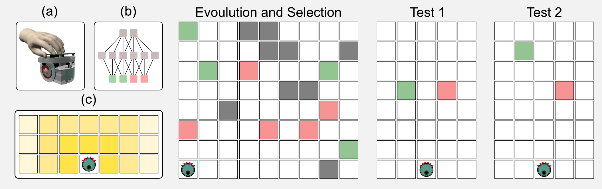
In the same period I was studying the decision making strategies of single robots in intertemporal choice tasks. Intertemporal choices concern options that can be obtained at different points in time: buying a luxury item today or saving the money to ensure a sizable pension in the future. In those experiments I used simulated e-puck robots [see figure (a)] which were controlled by a simple neural network [see figure (b)]. The sensors of the robot can localise the presence of two tokens: green and red. As you can see in figure (c) the sensors return a stronger signal when the token is close to the robot. The sensor signal is the input to the network, whereas the output is the speed of the two wheels of the robot. In a first phase the neural networks controlling the robots were evolved following an evolutionary strategy. The ratio of green (high energy) and red (low energy) tokens in the environment was manipulated, leading to rich and poor ecologies. In a second phase called the test phase, the robots had to choose between singles green or red tokens. The tokens were placed at the same distance from the robot but one of those was moved far away at each new trial. When the tokens were at the same distance from the robot it chose the highly energetic token. However moving the highly energetic token far away increased the preference for the less energetic one. The robot strategy changed based on the type of ecology used during the evolution. For example, poor ecologies increased the preference for the green token. This behaviour has been observed in many animals and especially in rats. It is incredible how simple neural networks evolved using GAs can represent such a sophisticated decision making strategy. If you are interested in this topic you can find more in the article I published with my colleagues: “Investigating intertemporal choice through experimental evolutionary robotics”. This is one of the practical applications of evolutionary algorithms.
I will start this post with an intuitive introduction which should help the reader who does not have familiarity with evolutionary methods. After the introduction I will dissect the main concepts behind GAs and we will give a look to some Python code. I will introduce many new terms because GAs have a slang which is different from the one used in reinforcement learning.
Evolutionary Algorithms (and birds)
The 27th of December 1831 the ship HMS Beagle sailed from Plymouth in England. Onboard there was Charles Darwin, the father of the theory of natural selection. The expedition was planned to last only two years, but it lasted for five. The Beagle visited Brasil, Patagonia, Strait of Magellan, Chile, Galapagos, etc. During the travel Darwin took notes about biology, geology and antropology of those places. Later on he published those notes in a book called “The voyage of the Beagle”. What did Darwin discovers during the travel?
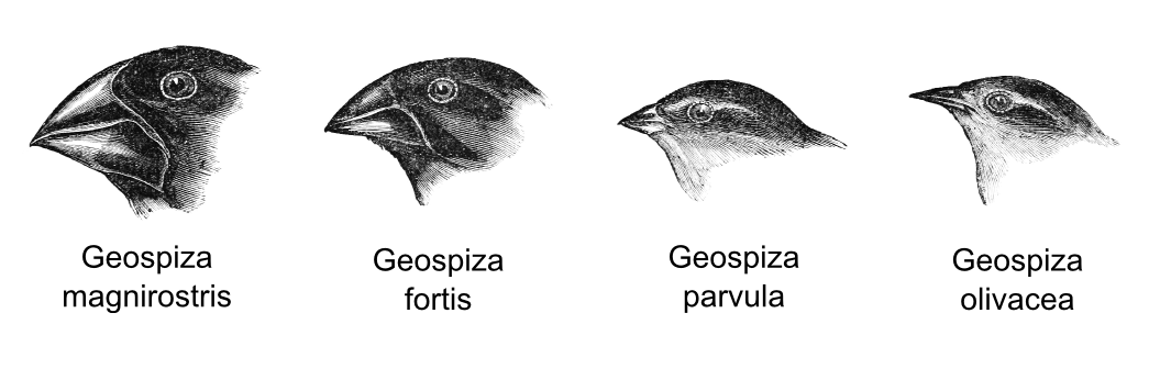
When visiting the Galapagos Darwin noticed the presence of some birds that appeared to have evolved from a single ancestral flock. Those birds shared common features but they were characterised by a remarkable diversity in beak form and function. Darwin hypothesised that the isolation of each species in a different small island was the cause of this high differentiation. In particular the shape of the beak evolved in accordance with the food availability on that island. Species with strong beak could eat hard seeds, whereas species with small beak preferred insects.
- Geospiza magnirostris: large size bird which can eat hard seeds.
- Geospiza fortis: medium size bird which prefer small and soft seeds.
- Geospiza parvula: small size bird which prefer medium size insects.
- Geospiza olivacea: small size bird which prefer to eat small insects.
Gradually Darwin found more and more proofs to this hypothesis and he eventually came out with the theory of natural selection. Today we call the Galapagos birds the Darwin’s finches. The Darwin’s finches are so isolated that it is possible to observe rapid evolution in a few generations when the environment changes. For example, the Geospiza fortis generally prefer soft seeds. However in the Seventies a severe drought reduced the supply of seeds. This finch was forced to turn to harder seeds which led in two generations to a 10% change in the size of the beak. What’s going on here? How can a population change so rapidly? How does natural selection operates?
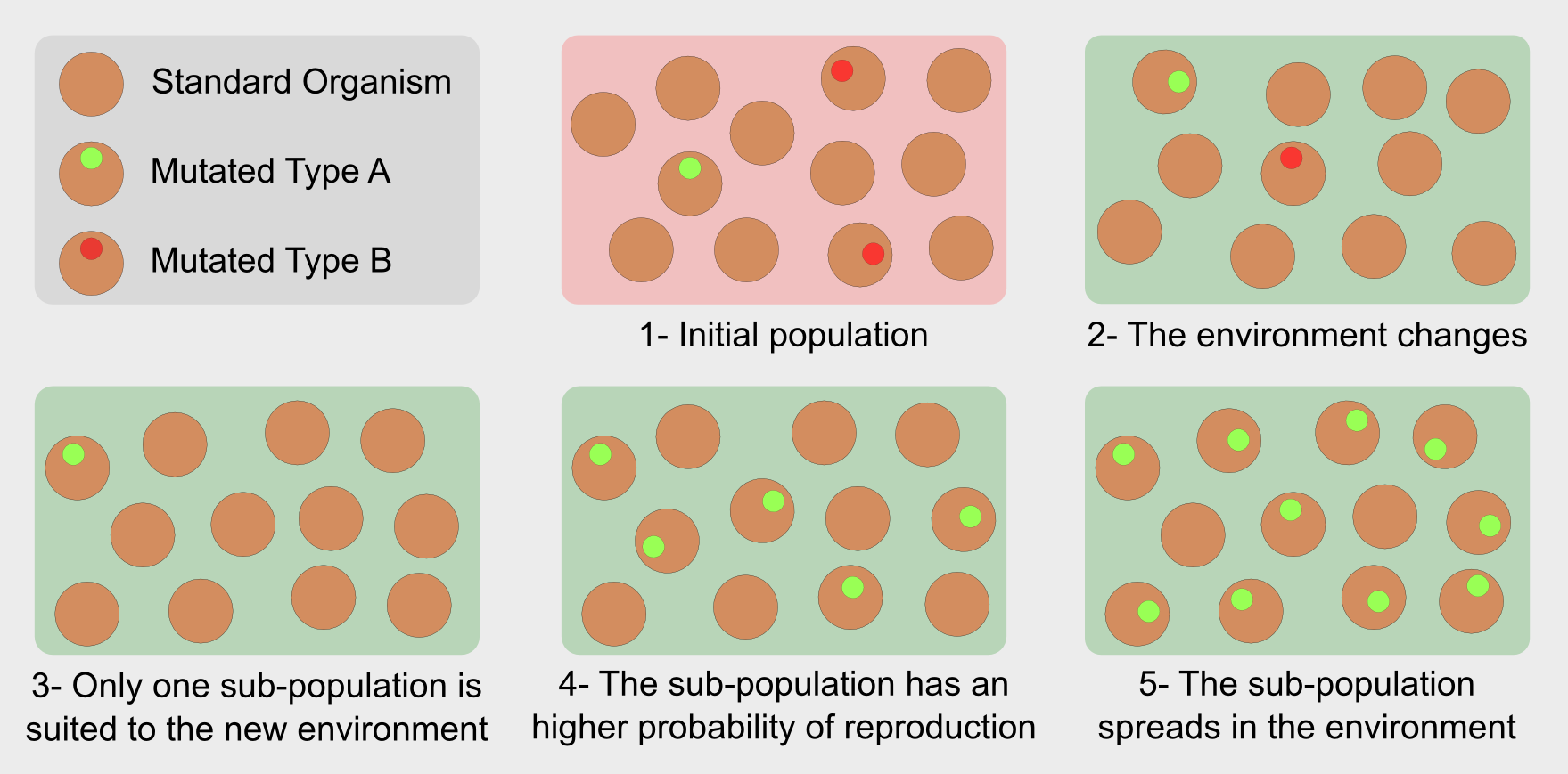
In the general population the individuals are the results of the crossover between two parents. The crossover is a form of recombination of the parents’ genetic material. In isolated populations redundancy of genetic material leads to very similar individuals. However it can happen that a random mutation modifies the newborn’s genotype generating organisms who carry on a new characteristic. For instance, in the Darwin’s finches it was a stronger beak. The mutation can bring an advantage for the subject, leading to a longer life and an higher probability of reproduction. On the other hand if the mutation does not carry any advantage it is discarded during the selection. That’s it. Evolution selects individuals with the variations best suited to a specific environment. In this sense evolution is not “the strongest survives” but “the fittest survives”.
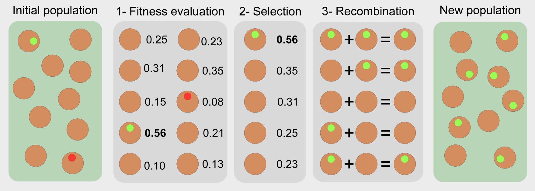
Evolutionary algorithms have features inspired by natural selection (reproduction, mutation, recombination, and selection). They are optimisers, meaning that they search for solutions to a problem directly in the solution space. The candidate solutions are single individuals like the Galapagos birds. In the standard approach a sequence of steps is used in order to evaluate and select the best solutions:
- Fitness function: it evaluates the performance of each candidate
- Selection: it chooses the best individuals based on their fitness score
- Recombination: it replicates and recombines the individuals
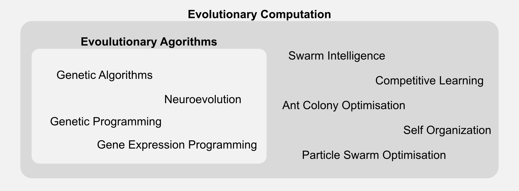
Evolutionary algorithms are part of a broader class called evolutionary computation. The generic label “evolutionary algorithm” applies to many techniques, which differ in representation and implementation details. Here I will focus only on genetic algorithms, however you should be aware that there are many variations out there.
In the next section I will introduce GAs which can be considered a special type of evolutionary algorithms. I will describe all the new terms and I will compare them to the ones encountered in the past episodes.
Genetic Algorithms
In the last section we saw how evolutionary algorithms works. In this section I will go deeper explaining how GAs work. As the name suggests GAs deals with genes. The metaphor of selection continue to works here but it is applied to genetic material. The idea is to describe each individual of the population with a specific genotype (or chromosome) which is used to express the individual’s features or phenotype. In biology the genotype represents the hereditary information of an organism and the phenotype is the observed features and behaviour of that organism. The distinction between genotype and phenotype and their interaction can be easily misunderstood. The genotype is only one of the factors that can influence the phenotype. Non-inherited factor and acquired mutations are not part of the genotype but have an influence on the phenotype. In GAs the genotype is usually represented by 1-D array where each value (sometimes called gene) represent a property.
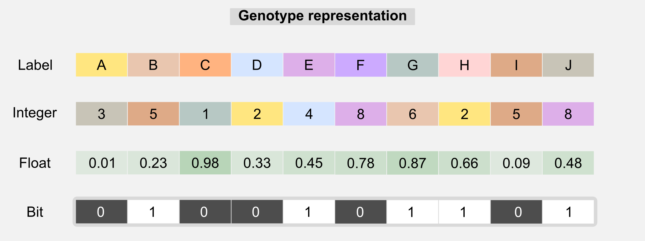
The genotype can contain labels, float, integers, or bits. Type uniformity in the chromosome is generally necessary in order to use the genetic operators. Label-based genotypes can be used in code-breaking. GAs can search in large solution spaces in order to get correct decryption. The integer-based genotypes are used in network topology optimisation. A float-based genotype can contain the weights of a neural network and those weights can be adjusted using GAs instead of backpropagation. This kind of optimisation is the one I used to evolve e-puck robots (see introduction). Choosing the right chromosome representation is generally up to the designer. Another thing that is up to the designer is the fitness function. The fitness function is the core of any GA and finding the right one is crucial. The fitness function gives an answer to the question: how close a given solution is to achieve the objectives? In many applications there are multiple fitness functions we can use. For example, if we are evolving a controller for a drone then the fitness function can be defined by how long the drone remains in the air. However this function does not incorporate any information about the stability of the flight. A better one can take into account the values returned by the inertial unit giving higher score to controllers which have more stability. The choice of the correct fitness function may require certain experience with GAs, however for many problems also an approximate fitness can lead to good solutions. In the next section I will show you how the fitness function is related to the concept of reward in reinforcement learning. Now it’s the moment to describe all the operators available in GAs and how they are used in the evolution process.
Selection: the selection is a way to reduce the number of possible solutions choosing the one that leads to the best results. After fitness evaluation it is possible to order the chromosomes from best to worst. The ordered list is then used by the selection mechanism. There are different types of selection. Truncated selection is the simplest form of selection. Only a fraction of the total number of chromosomes is selected, the rest is rejected.
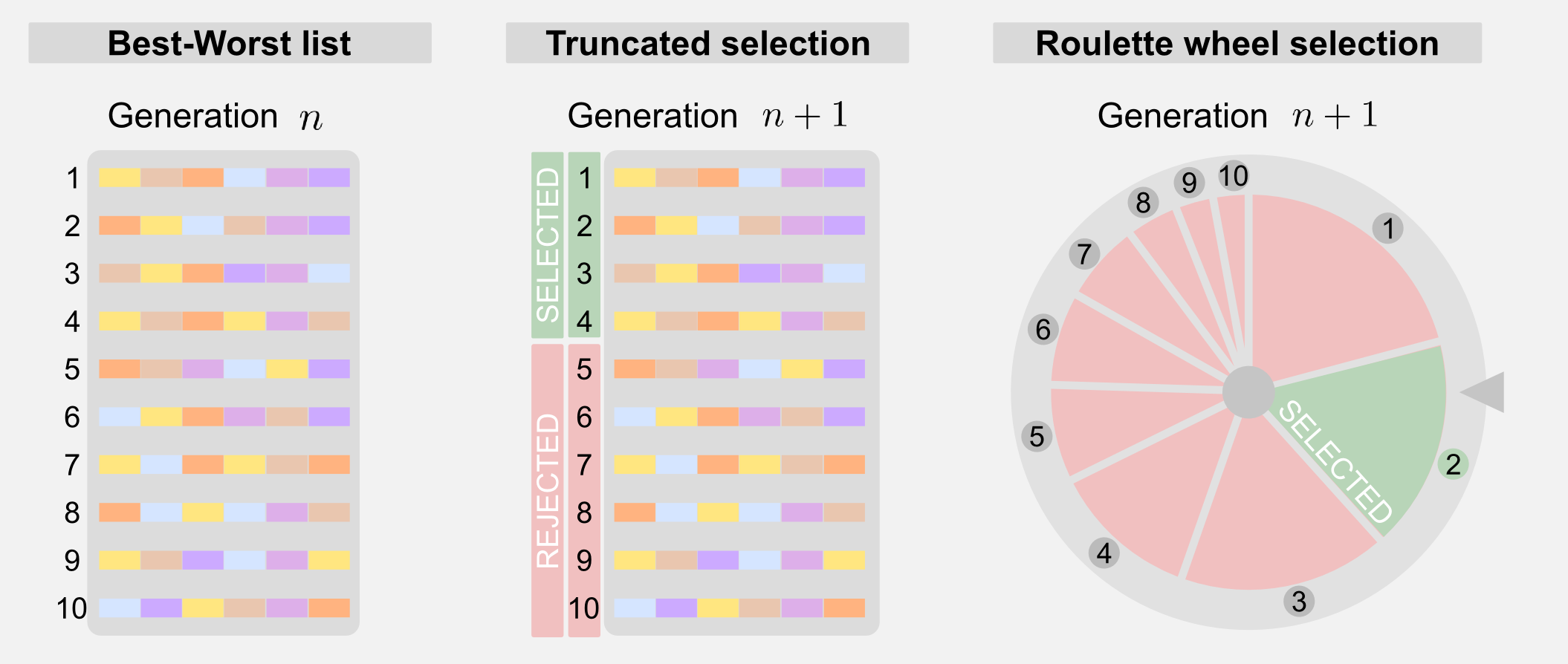
A more sophisticated form of selection is called roulette wheel. To each chromosomes is given a weight and this weight corresponds to a portion of a roulette wheel. Chromosomes with higher fitness will have higher weight and a larger portion of the wheel. Spinning the wheel for different times allows selecting the individuals for the next generation. The roulette wheel is nothing more than a weighted sort mechanism. You must notice that using the roulette wheel the same chromosome can be sorted multiple times and the probability of its presence in the next generation is higher. Another form of selection is called tournament selection and it consists in randomly selecting a group of individuals and taking only the one with the highest fitness.
The selection process can mark a few individuals as elite, meaning that their genotype will be copied without variations in the new generation. This mechanism is called elitism and is used to keep the best solutions into the evolutionary loop. I will use elitism in the python implementation, an example will give you a wider view on its function.
Mutation: this operator is used in order to avoid uniformity in the population. The mutation randomly changes one value of the genotype. The mutation allows avoiding local minima in the search space, randomly changing the existing solutions. The simplest version of the mutation is called point mutation and is similar to the biological mechanism that operates on DNA.
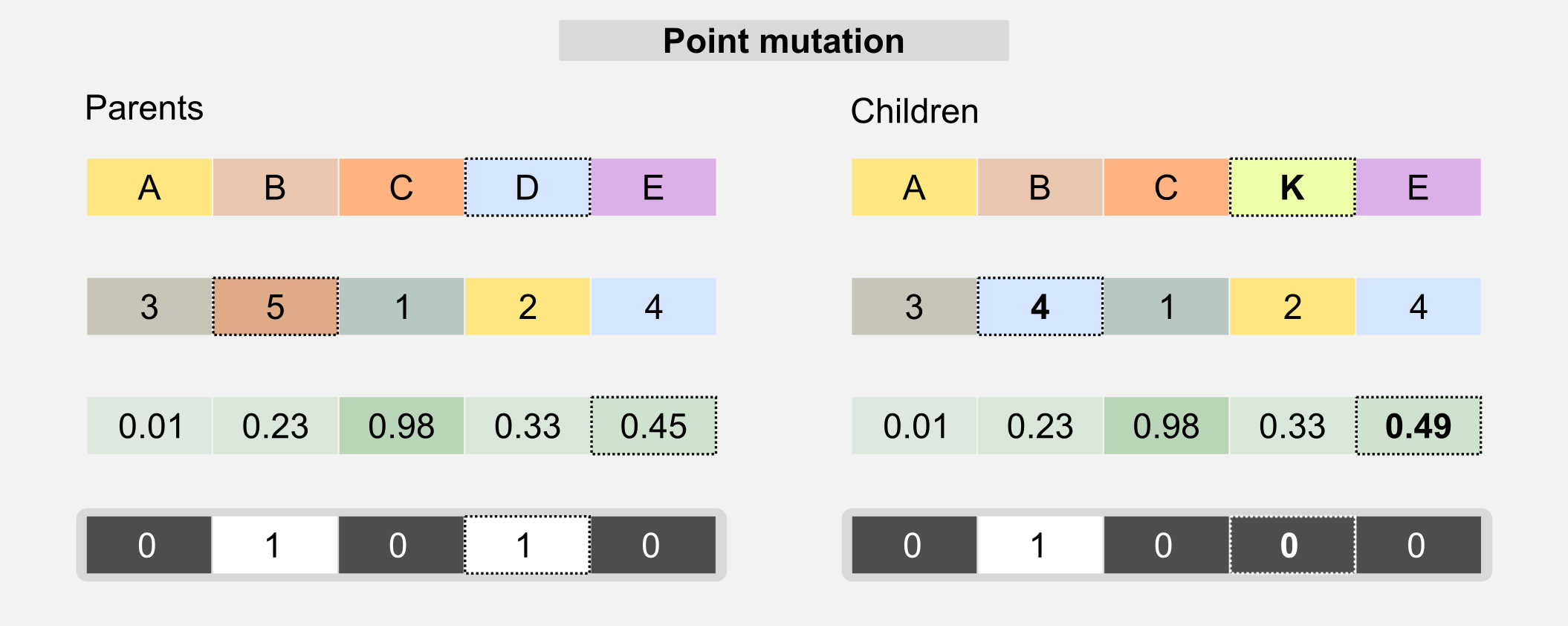
The probability of a mutation is generally described by a mutation rate which must be carefully selected. A high mutation rate can lead to the loss of the best individuals, whereas a low mutation rate leads to genotypes uniformity. For label and integer-based chromosomes, the mutation changes a single gene to a value randomly picked from a predefined set. For bit-based chromosomes the value of the gene is switched to its opposite when the mutation happens. In float-based chromosomes the value can be sampled from a uniform distribution or from a Gaussian distribution centred on the gene value.
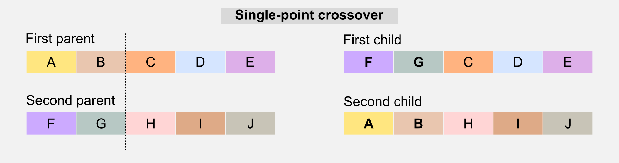
Crossover: this operator is similar to the biological counterpart and it is used to recombine the genotype of the parents to generate offspring who have mixed features. The simplest form of crossover is called single-point. Given the two parents’ genotypes and a random slicing point, the single-point crossover literally “cross” the two portions when generating the children.
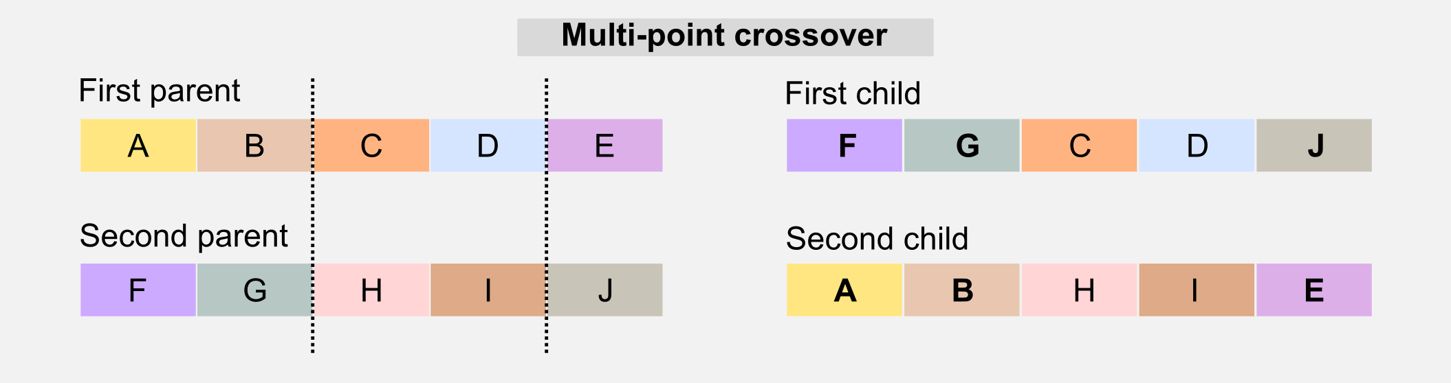
Another version of the crossover is called multi-point crossover. The multi-point crossover selects multiple slicing points and recombines those parts in the children’s genotype.
There are other crossover solutions that involve multiple parents, however in the next sections I will focus only on the single-point version.
GAs in reinforcement learning
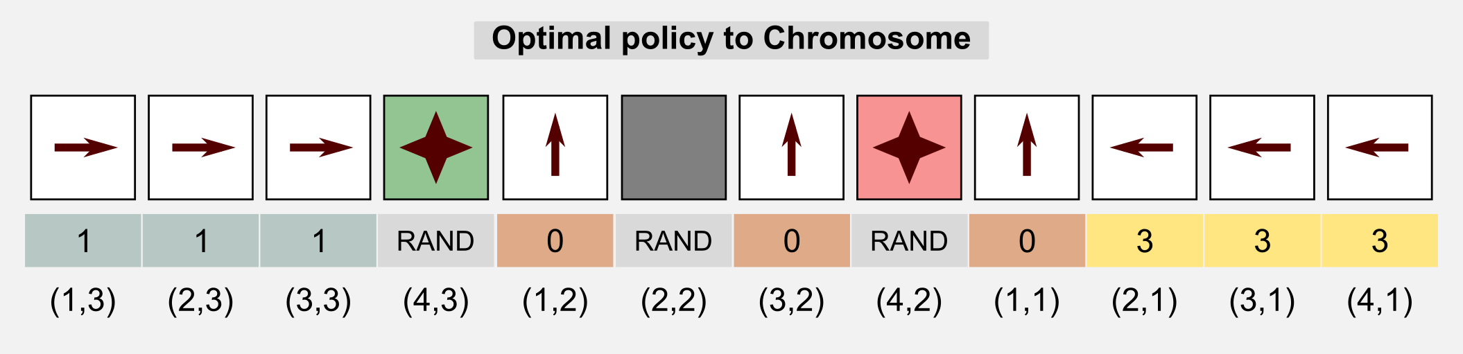
How can we use GAs in reinforcement learning? GAs can be used for policy estimation. In this case the 1-D genotype is a representation of the policy matrix. In the following sections I will use the words genotype and chromosome interchangeably. As usual I will start from the cleaning robot example introduced in the first post. A cleaning robot can move in a 4x3 discrete world. The reward for each state is -0.04 but for the charging station (+1.0) and the stairs (-1.0). The environment is not deterministic and each action taken by the robot has 20% probability of failure. The optimal policy for this environment is given. Here we want to see if the GAs can obtain the optimal policy through recombination of the population chromosomes. We can use an integer-based representation where for each number there is a corresponding action: 0=UP, 1=RIGHT, 2=DOWN, 3=LEFT. For terminal states and obstacles we do not really need an action, because in these states the action does not take place. For this reason we can represent the action using a random value or we can discard those states from the chromosome. Here for the sake of clarity I choose the first solution.
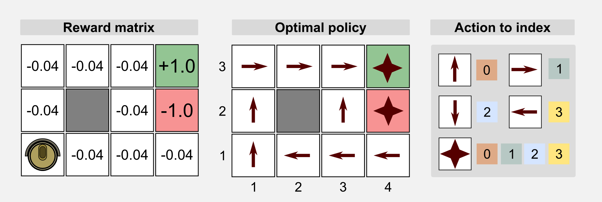
We can represent the genotype as the unrolled policy matrix which associate an action to each state. Starting from the state (1,1) (columns x rows) and following the Russel and Norvig convention for the grid world (the starting point is in the bottom-left corner) we associate to each action an index and we store each value in the chromosome.
The starting population will have random initialised genotypes, meaning that the behaviour of each robot will be different. The fitness score allow us to discriminate between good and bad policies. Here the fitness value is defined as the sum of rewards obtained at each time step \(t\) for all the \(M\) episodes:
\[\text{Fitness} = \sum_{e=0}^{M} \sum_{t=0}^{N} r_{t}^{(e)}\]The chromosome is evaluated on multiple episodes in order to have a better estimation of its performance. Here the exploring start condition is necessary in order to guarantee a wide exploration of the search space. We can summarise everything in two points:
- The genotype (or chromosome) represents the policy matrix
- The fitness score represents the cumulated reward in multiple episodes
It is interesting to understand how the genetic operators modify the chromosomes/policy. The mutation randomly modifies the action taken in a particular state. This operator guarantees the exploration of the solution space. The crossover takes two chromosomes and mixes them. Let’s suppose we have two parents. The first one represents a policy which is particularly good in the upper part of the grid world but not so good in the lower part. The second parent represents a policy which is good in the lower part but it is really bad in the upper. Mixing these two chromosomes through a single-point crossover generates two children, one which is very good and the other which is very bad. Now it’s time to implement everything in Python.
Python implementation
The Python implementation is built upon different functions that represent the genetic operators described above. First of all we need a function to generate a random population of chromosomes. Using the Numpy method numpy.random.choice() it can be done in one line. Each value of the chromosome is a gene which is picked from a predefined set. In our case the set is represented by the four discrete actions the robot can take [0, 1, 2, 3].
def return_random_population(population_size, chromosome_size, gene_set):
    '''Returns a random initialised population

    This funtion initialise a matrix of integers using numpy randint.
    @param chromosome_size
    @param population_size
    @param gene_set list or array containing the gene values
    @return matrix of integers size:
         population_size x chromosome_size
    '''
    return np.random.choice(gene_set,
                            size=(population_size,chromosome_size))
Once the random population is ready we can estimate the fitness for each individual obtaining a fitness array. We need a function to sort the chromosomes in best-worst order. In Numpy the method numpy.argsort() returns the position of the values inside an array from the lowest to the highest (worst-best). This method is particularly efficient because by default it uses the quicksort algorithm. In the last step we have to reverse the order of the elements to obtain the best-worst list we were looking for. Everything can be implemented in Python in a few lines:
def return_best_worst_population(population, fitness_array):
    '''Returns the population sorted in best-worst order

    @param population numpy matrix containing the population chromosomes
    @param fitness_array numpy array containing the fitness score for
        each chromosomes
    @return the new population and the new fitness array
    '''
    new_population = np.zeros(population.shape)
    new_fitness_array = np.zeros(fitness_array.shape)
    worst_best_indeces = np.argsort(fitness_array)
    best_worst_indeces = worst_best_indeces[::-1] #reverse the array
    row_counter = 0
    for index in best_worst_indeces:
         new_population[row_counter,:] = population[index,:]
         new_fitness_array[row_counter] = fitness_array[index]
         row_counter += 1
    return new_population, new_fitness_array
Once we have the sorted population is then possible to select the best individuals.
The truncated selection mechanism can be implemented using the Numpy method numpy.resize() that takes as input a matrix and returns part of it.
def return_truncated_population(population, fitness_array, new_size):
     '''Truncates the input population and returns part of the matrix

     @param population numpy array containing the chromosomes
     @param fitness_array numpy array containing the fitness score for
         each chromosomes
     @param new_size the size of the new population
     @return a population containing new_size chromosomes
     '''
     chromosome_size = population.shape[1]
     pop_size = population.shape[0]
     new_population = np.resize(population, (new_size,chromosome_size))
     new_fitness_array = np.resize(fitness_array, new_size)
     return new_population, new_fitness_array
In the previous sections I showed another selection mechanism, the roulette wheel. The roulette wheel can be implemented easily using the Numpy method numpy.random.choice() which can take as input an array representing the probabilities associated with each element of the input array. Because the probabilities must sum up to one we have to normalise the values contained in the fitness array using a softmax function.
def return_roulette_selected_population(population, fitness_array, new_size):
  '''Returns a new population of individuals (roulette wheel).

  Implementation of a roulette wheel mechanism. The population returned
  is obtained through a weighted sampling based on the fitness array.
  @param population numpy matrix containing the population chromosomes
  @param fitness_array numpy array containing the fitness score for
      each chromosomes
  @param new_size the size of the new population
  @return a new population of roulette selected chromosomes, and
          the fitness array reorganised based on the new population.
  '''
  #Softmax to obtain a probability distribution from the fitness array.
  fitness_distribution = np.exp(fitness_array -
                         np.max(fitness_array))/np.sum(np.exp(fitness_array -
                                                       np.max(fitness_array)))
  #Selecting the new population indeces through a weighted sampling
  pop_size = population.shape[0]
  chromosome_size = population.shape[1]
  pop_indeces = np.random.choice(pop_size, new_size, p=fitness_distribution)
  #New population initialisation
  new_population = np.zeros((new_size, chromosome_size))
  new_fitness_array = np.zeros(new_size)
  #Assign the chromosomes in population to new_population
  row_counter = 0
  for i in pop_indeces:
      new_population[row_counter,:] = np.copy(population[i,:])
      new_fitness_array[row_counter] = np.copy(fitness_array[i])
      row_counter += 1
  return new_population, new_fitness_array
The next step of the GA is the crossover function. There are different ways to implement crossover. Here the parents are randomly sampled from the input population and a new population of new_size chromosomes is created. In this simplified version two parents generate only one child. A slicing point is randomly defined. The first part of the child’s chromosome contains the first parent genes while the second part is taken from the second parent. The elite parameter defines how many individuals are copied in the new population without being crossed. When using the elitism the population must be sorted from best to worst.
def return_crossed_population(population, new_size, elite=0):
    '''Return a new population based on the crossover of the individuals

    The parents are randomly chosen. Each pair of parents generates
    only one child. The slicing point is randomly chosen.
    @param population numpy matrix containing the population chromosomes
    @param new_size defines the size of the new population
    @param elite defines how many chromosomes remain unchanged
    @return a new population of crossed individuals
    '''
    pop_size = population.shape[0]
    chromosome_size = population.shape[1]
    if(elite > new_size):
        ValueError("Error: the elite value cannot " +
                    "be larger than the population size")
    new_population = np.zeros((new_size,chromosome_size))
    #Copy the elite into the new population matrix
    new_population[0:elite] = population[0:elite]
    #Randomly pick the parents to cross
    parents_index = np.random.randint(low=0,
                                      high=pop_size,
                                      size=(new_size-elite,2))
    #Generating the remaining individuals through crossover
    for i in range(elite,new_size-elite):
        first_parent = population[parents_index[i,0], :]
        second_parent = population[parents_index[i,1], :]
        slicing_point = np.random.randint(low=0, high=chromosome_size)
        child = np.zeros(chromosome_size)
        child[0:slicing_point] = first_parent[0:slicing_point]
        child[slicing_point:] = second_parent[slicing_point:]
        new_population[i] = np.copy(child)
    return new_population
Finally the mutation operator. The mutation iterates through all the values of all the chromosomes and for each value randomly mutates the content picking an integer from a predefined set. In our case the set represents the four actions available to the robot [0, 1, 2, 3]. We can iterate over Numpy array using the function numpy.nditer() changing the value of an element only if a random float picked from a uniform distribution is less than mutation_rate. The elite parameter represents the number of individual in the population matrix to keep unchanged. As I explained in the previous section the elitism is useful for saving the best solutions ever.
def return_mutated_population(population, gene_set, mutation_rate, elite=0):
    '''Returns a mutated population

    It applies the point-mutation mechanism to each value
    contained in the chromosomes.
    @param population numpy array containing the chromosomes
    @param gene_set a numpy array with the value to pick
    @parma mutation_rate a float repesenting the probaiblity
        of mutation for each gene (e.g. 0.02=2%)
    @return the mutated population
    '''
    for x in np.nditer(population[elite:,:], op_flags=['readwrite']):
        if(np.random.uniform(0,1) < mutation_rate):
            x[...] = np.random.choice(gene_set, 1)
    return population
Now we have to stick everything together and see what we get. The first thing to do is to define some hyper-parameters we can play with. Different results can be obtained by modifying each one of these parameters. Increasing tot_episodes you will get a better estimation of the fitness. The tot_steps defines how many steps are allowed for each episode. A good value for the girdworld is given by the number of rows plus the number of columns times two. The population_size should be increased accordingly with the state space. A larger space may require more individuals. The elite_size generally corresponds to 10% of the total population. This parameter should not be too high otherwise the population will be too uniform. The mutation_rate is really important. Here I used a value of 10% but a lower probability of 5% is generally used. I invite you to run the script with different parameters and see what happens.
The gene_set and chromosome_size are parameters which are specific to the 4x3 gridworld. You should modify them if you want to reuse the code in another application.
tot_generations = 100
tot_episodes = 100
tot_steps = 14
population_size = 100
elite_size = 10
mutation_rate = 0.10
gene_set = [0, 1, 2, 3]
chromosome_size = 12
After defining the hyper-parameters we have to generate the initial population. For the 4x3 gridworld it is enough to have a population of 100 chromosomes which can be randomly initialised with the return_random_population() function. After that it is time to setup the main loop. Each chromosome is evaluated for 100 episodes with exploring_starts condition set to true. The fitness is accumulated along all the episodes. After the fitness evaluation the first step is the selection. Here the line for the roulette wheel selection is commented because I will use a simple truncated selection taking only half of the population.
for generation in range(tot_generations):
  #The fitness value for each individual is stored in np.array
  fitness_array = np.zeros((population_size))
  for chromosome_index in range(population_size):
    for episode in range(100):
      #Reset and return the first observation
      observation = env.reset(exploring_starts=True)
      for step in range(30):
        #Estimating the action for that state
        col = observation[1] + (observation[0]*world_columns)
        action = population_matrix[chromosome_index,:][col]
        #Taking the action and observing the new state and reward
        observation, reward, done = env.step(action)
        #Accumulating the fitness for this individual
        fitness_array[chromosome_index] += reward
        if done: break

  #Uncomment the following lines to enable roulette wheel selection
  #population_matrix, fitness_array = \
    #return_roulette_selected_population(population_matrix,
                                        #fitness_array,
                                        #population_size)
  population_matrix, fitness_array = \
    return_best_worst_population(population_matrix, fitness_array)
  #Comment the following line if you enable the roulette wheel
  population_matrix, fitness_array = \
    return_truncated_population(population_matrix,
                                fitness_array,
                                new_size=int(population_size/2))
  population_matrix = return_crossed_population(population_matrix,
                                                population_size,
                                                elite=10)
  population_matrix = return_mutated_population(population_matrix,
                                                gene_set=[0,1,2,3],
                                                mutation_rate=mutation_rate,
                                                elite=10)
As usual the full code is available in my GitHub repository and is called genetic_algorithm_policy_estimation.py. I set mutation_rate=0.10 and elite_size=10. Launching the script will give you the average fitness score, and the score of the best and worst individual for each generation.
Generation: 1
Fitness Mean: -94.4964
Fitness STD: 35.5458518964
Fitness Max: 18.24 at index 57
Fitness Min: -142.2 at index 79

Generation: 2
Fitness Mean: -63.348
Fitness STD: 32.8610677855
Fitness Max: 20.64 at index 71
Fitness Min: -116.6 at index 46

Generation: 3
Fitness Mean: -46.9696
Fitness STD: 35.4612189841
Fitness Max: 41.36 at index 60
Fitness Min: -127.32 at index 37

...

Generation: 10
Fitness Mean: 17.7552
Fitness STD: 56.6485542354
Fitness Max: 75.4 at index 1
Fitness Min: -131.72 at index 72

...

Generation: 50
Fitness Mean: 35.9964
Fitness STD: 54.7041918964
Fitness Max: 83.84 at index 26
Fitness Min: -122.64 at index 21

...

Generation: 100
Fitness Mean: 39.4068
Fitness STD: 53.0702770462
Fitness Max: 82.36 at index 55
Fitness Min: -126.0 at index 22
How should we interpret this information? When the selection mechanism is working the average fitness increases. In our case we can see that it passes from -94.5 of the first generation to -47.0 in the third, eventually reaching a score of 39.4 in the hundredth. The score of the best and worst individuals can be shaky because those individuals are outliers and their performance can have a large variance. For the best and worst individual you can see the corresponding index in the fitness array. The index is useful for understanding if the best individual is part of the elite (in our case the first 10 subjects) or not. When the individual is not part of the elite it means that the genetic operators managed to find a better solution outside of the elite circle. For example, in generation 10 the highest fitness has been obtained by the first individual, while in the generation 50 by the individual number 26. In the first case the best was part of the elite, in the second case it was not.
The standard deviation is an important indicator because it can tell us if there is genetic redundancy in the population. When the standard deviation is low it means that the individuals have similar performances and probably this is due to uniformity in the chromosomes. During the evolution you may see the standard deviation increasing, this indicates that the variance is getting larger due to the multiplication of branches in the individual’s genotype.
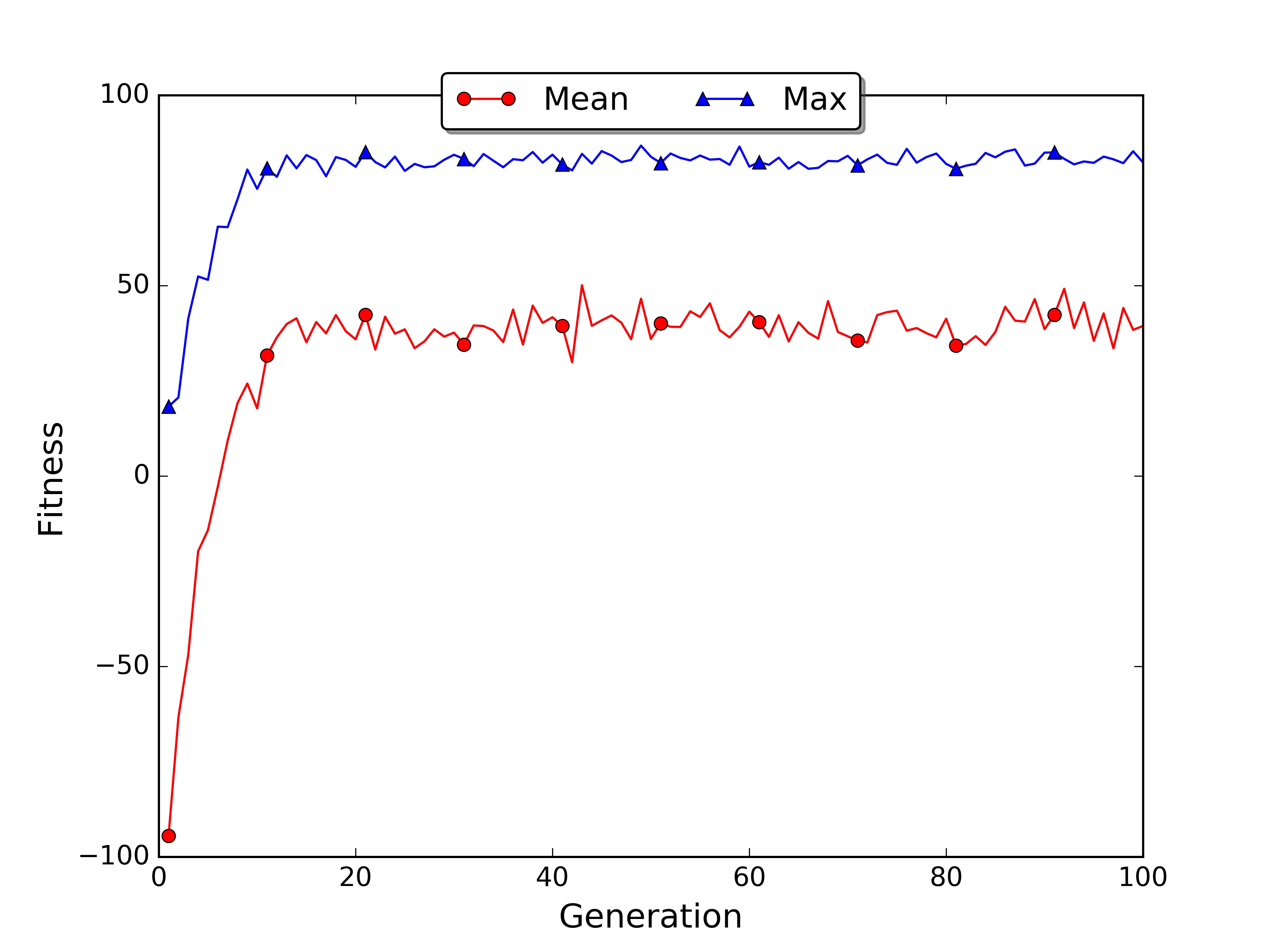
If you have matplotlib installed the script will automatically save the plot of the best and average fitness for each generation in the file fitness.jpg. In my case the average fitness went up in the first 20 generations and then reached a plateau. Uncommenting the roulette wheel line and commenting the truncated selection line we can get the plot for the roulette wheel selection.
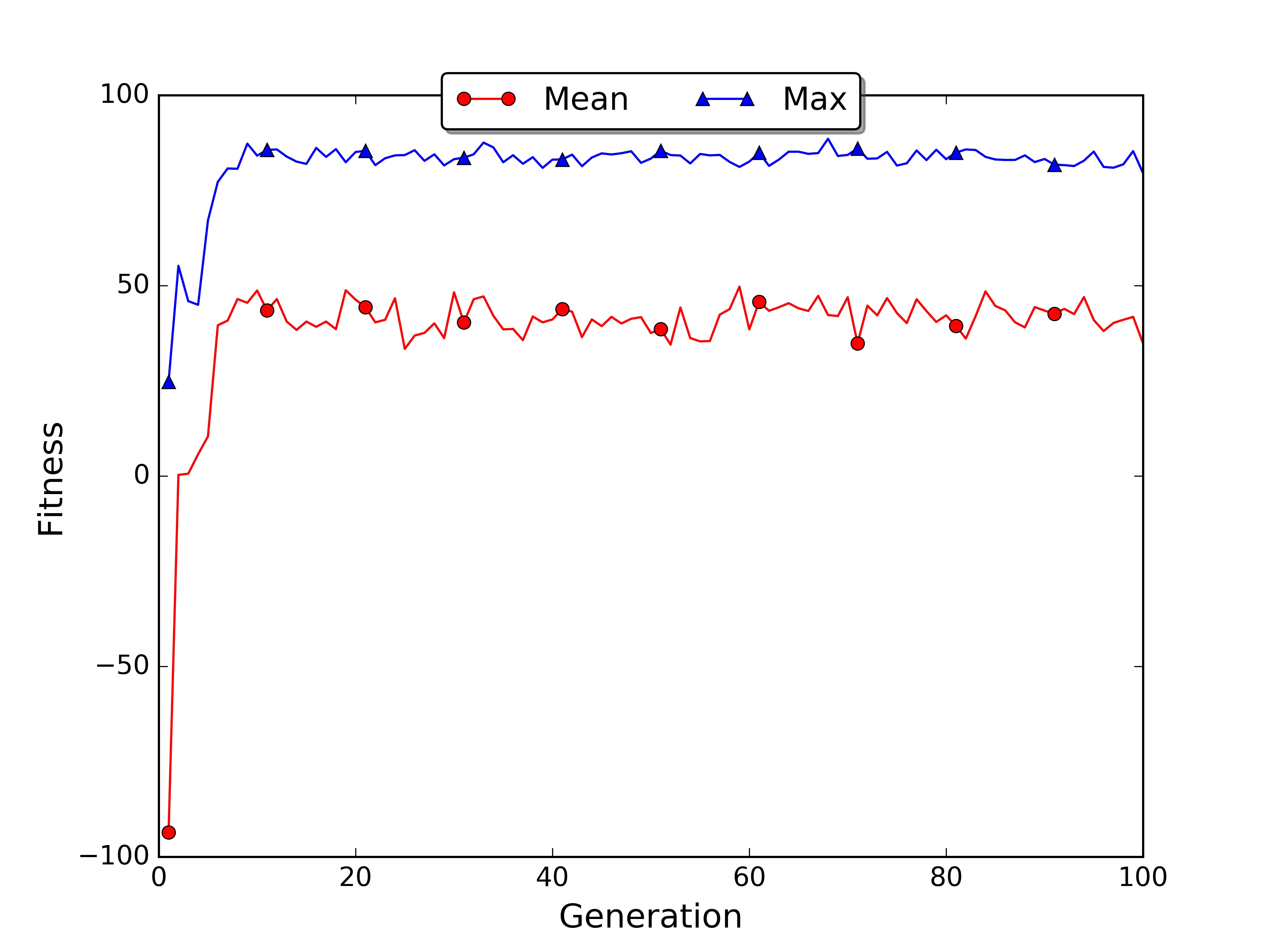
In the roulette wheel plot the average fitness grows faster because the sampling mechanism moved to the next generation an higher number of good policies.
It is interesting to have a look to the elite (first 10 individuals) to see which kind of policy they adopted. In my simulation at generation 100 most of the elite’s chromosomes are optimal or sub-optimal.
Optimal Policy:
 >  >  >  *  ^  #  ^  *  ^  <  <  <

Chromosome 1:
 >  >  >  *  ^  #  ^  *  ^  >  ^  <
Chromosome 2:
 >  >  >  *  ^  #  ^  *  ^  <  <  <
Chromosome 3:
 >  >  >  *  ^  #  ^  *  ^  <  ^  <
Chromosome 4:
 >  >  >  *  ^  #  ^  *  ^  >  ^  <
Chromosome 5:
 >  >  >  *  ^  #  ^  *  ^  <  <  <
Chromosome 6:
 >  >  >  *  ^  #  ^  *  ^  ^  ^  <
Chromosome 7:
 >  >  >  *  ^  #  ^  *  ^  v  ^  <
Chromosome 8:
 >  >  >  *  ^  #  ^  *  ^  >  ^  <
Chromosome 9:
 >  >  >  *  ^  #  ^  *  ^  <  ^  <
Chromosome 10:
 >  >  >  *  ^  #  ^  *  ^  <  <  <
If we scale up the example on a 30x10 gridworld everything gets harder. In the GitHub repository you will find another file called genetic_algorithm_policy_estimation_large_world.py where the gridworld has dimension 30x10. You can re-adapt the script to different worlds changing the environment initialisation, the chromosome_size and the parameter tot_steps. I kept population_size and tot_episodes equal to 100 and I run the script for 300 generations.
Generation: 1
Fitness Mean: -313.6372
Fitness STD: 6.56887997759
Fitness Max: -289.44 at index 3
Fitness Min: -320.32 at index 38

Generation: 2
Fitness Mean: -307.286
Fitness STD: 11.1612836179
Fitness Max: -265.88 at index 99
Fitness Min: -321.2 at index 56

Generation: 3
Fitness Mean: -301.32
Fitness STD: 13.0532141636
Fitness Max: -265.24 at index 2
Fitness Min: -320.0 at index 12

...

Generation: 100
Fitness Mean: -236.0288
Fitness STD: 42.1012775407
Fitness Max: -143.88 at index 4
Fitness Min: -320.0 at index 70

...

Generation: 300
Fitness Mean: -220.7844
Fitness STD: 52.0733055283
Fitness Max: -111.16 at index 31
Fitness Min: -320.0 at index 43
The training took almost 2 hours while for the small world only a few minutes. The average and max fitness increased slowly during the generations. The plot allows visualising the general trend, showing that there is room for improvement. If you want you can run the script for more generations and see when the fitness reaches a plateau.
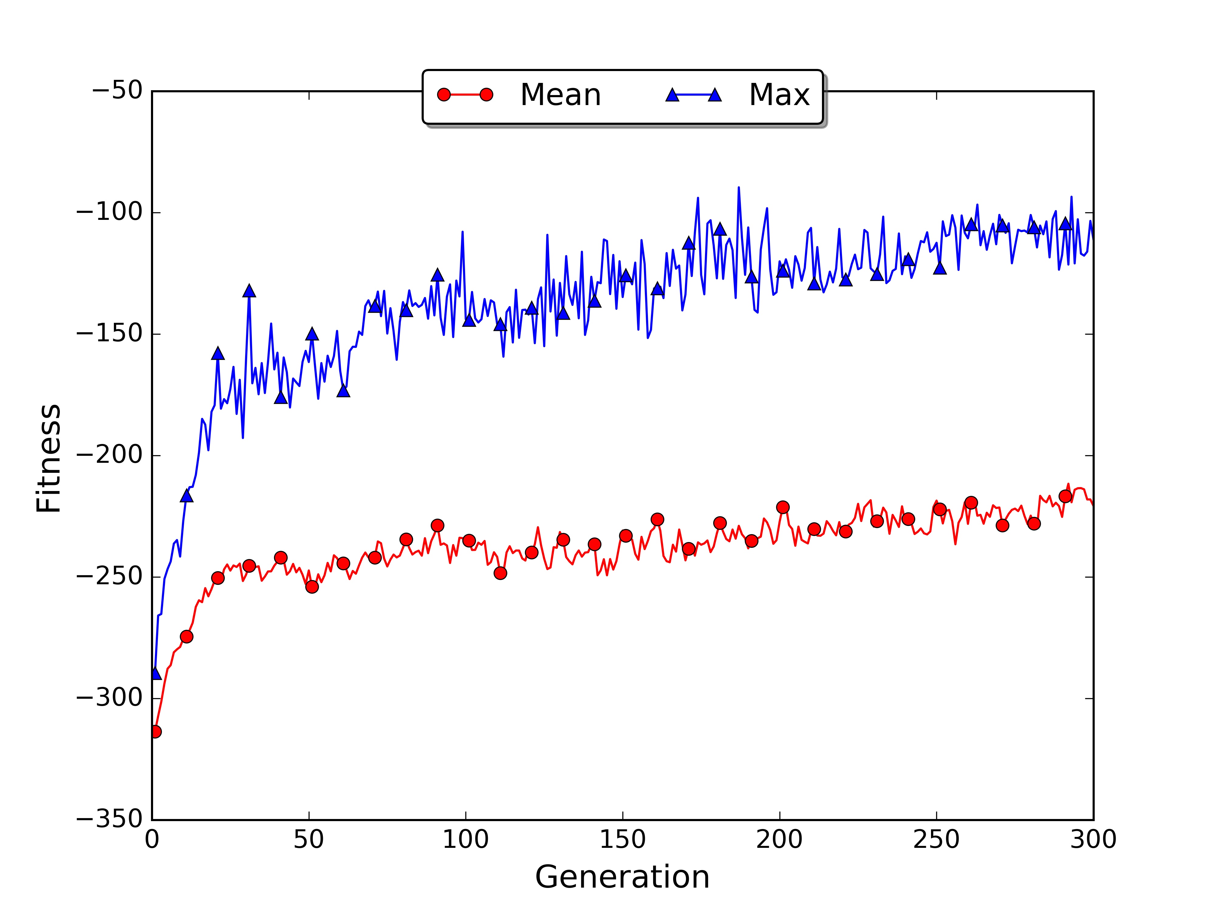
As you noticed with the large world example the limit of the genetic approach is that it may need many generations in order to converge. Moreover it cannot learn online as we saw in temporal differencing learning. For these reasons GAs are generally used in simulated environments, where multiple instances of the world can run in parallel and are not computationally expensive.
Conclusions
In this post I introduced evolutionary and genetic algorithms. GAs are based on the natural selection mechanism and they can be used to search for policies directly in the policy space. In reinforcement learning the use of GAs can be advantageous when the state of the Markov decision process is partially hidden or misperceived. The python code I released with this post is generic and can be applied to a large variety of problems. Feel free to reuse it for your own applications. Moreover online you will find simulators based on GAs that can run on your browser, you can find a couple of example in the resources section.
This post can be considered the conclusion of the first part of the series. We are ready to apply the knowledge accumulated until now to more complex problems. Reinforcement learning is a great tool and it can be used in many scenarios, in the next post I will show you its potential.
Acknowledgments
The e-puck picture is taken from the cyberbotics website here
Index
- [First Post] Markov Decision Process, Bellman Equation, Value iteration and Policy Iteration algorithms.
- [Second Post] Monte Carlo Intuition, Monte Carlo methods, Prediction and Control, Generalised Policy Iteration, Q-function.
- [Third Post] Temporal Differencing intuition, Animal Learning, TD(0), TD(λ) and Eligibility Traces, SARSA, Q-learning.
- [Fourth Post] Neurobiology behind Actor-Critic methods, computational Actor-Critic methods, Actor-only and Critic-only methods.
- [Fifth Post] Evolutionary Algorithms introduction, Genetic Algorithms in Reinforcement Learning, Genetic Algorithms for policy selection.
- [Sixt Post] Reinforcement learning applications, Multi-Armed Bandit, Mountain Car, Inverted Pendulum, Drone landing, Hard problems.
- [Seventh Post] Function approximation, Intuition, Linear approximator, Applications, High-order approximators.
- [Eighth Post] Non-linear function approximation, Perceptron, Multi Layer Perceptron, Applications, Policy Gradient.
Resources
-
The complete code for the Genetic Algorithm examples is available on the dissecting-reinforcement-learning official repository on GitHub.
-
Scholarpedia article on Neuroevolution [web]
-
Genetic algorithm walkers simulator [web]
-
Genetic algorithm cars simulator [web]
-
List of genetic algorithm applications [wiki]
-
Evolutionary Algorithms for Reinforcement Learning. Moriarty, D. E., Schultz, A. C., & Grefenstette, J. J. (1999). [pdf]
-
Reinforcement learning: An introduction (Chapter 1.3) Sutton, R. S., & Barto, A. G. (1998). Cambridge: MIT press. [html]
-
Evolution Strategies as a Scalable Alternative to Reinforcement Learning Salimans, T., Ho, J., Chen, X., & Sutskever, I. (2017). arXiv preprint arXiv:1703.03864. [pdf]
References
Goldberg, D. E., & Holland, J. H. (1988). Genetic algorithms and machine learning. Machine learning, 3(2), 95-99.
Mitchell, M. (1998). An introduction to genetic algorithms. MIT press.
Moriarty, D. E., Schultz, A. C., & Grefenstette, J. J. (1999). Evolutionary algorithms for reinforcement learning. J. Artif. Intell. Res.(JAIR), 11, 241-276.
Paglieri, F., Parisi, D., Patacchiola, M., & Petrosino, G. (2015). Investigating intertemporal choice through experimental evolutionary robotics. Behavioural processes, 115, 1-18.
Salimans, T., Ho, J., Chen, X., & Sutskever, I. (2017). Evolution Strategies as a Scalable Alternative to Reinforcement Learning. arXiv preprint arXiv:1703.03864.