Playing the Google Chrome's dinosaur game using hand-tracking

Today I was looking for some robust/fast way to track hands in OpenCV. At the beginning I turned my attention to classifiers such as: Haar cascade, Convolutional Neural Networks, SVM, etc. Unfortunately there are two main problems with classifiers: slinding windows and datasets.

1. To classify parts of an image it is often used a standard approach called sliding window. A sliding window is a window of predefined size that is moved over an image and which content is given as input to the classifier. This approach is widely used in computer vision but it has a drawback, it is slow and it can require many iterations to find all the objects in the image.

2. Another problem when you want to implement a classifier is to find datasets which can be used in the training phase. OpenCV has an Haar cascade classifier for hand detection but it has been trained on a limited dataset and it recognises hands in predefined poses.

Given this two problems, what to do? One possibility is to use the histogram backprojection algorithm.

The histogram backprojection algorithm

The histogram backprojection algorithm was proposed by Swain and Ballard in their article “Color Indexing”. If you did not read my previous post about histogram intersection you should do it, since backprojection can be considered complementary to intersection. Using the terminology of Swain and Ballard we can say that the intersection answers to the question “What is the object we are looking to?”, whereas the backprojection answers to the question “Where in the image are the colors that belong to the object being looked for (the target)?”. How does the backprojection work? Given the image histogram \(I\) and the model histogram \(M\) we define a ratio histogram \(R\) as follow:

\[R_{i} = min \bigg( \frac{M_{i}}{I_{i}}, 1 \bigg)\]

We define also a function \(h(c)\) that maps the colour \(c\) of the pixel at \((x, y)\) to the value of the histogram \(R\) it indexes. Using the slang of Swain and Ballard we can say that the function \(h(c)\) backprojects the histogram \(R\) onto the input image. The backprojected image \(B\) is then convolved with a disk \(D\) of radius \(r\). The authors recommend to choose as area of \(D\) the expected area subtended by the object. If you want more technical details I suggest you to read the original article which is not so long and it is well written. Since the backprojection process can be hard to grasp I realised an image which explain what’s going on:

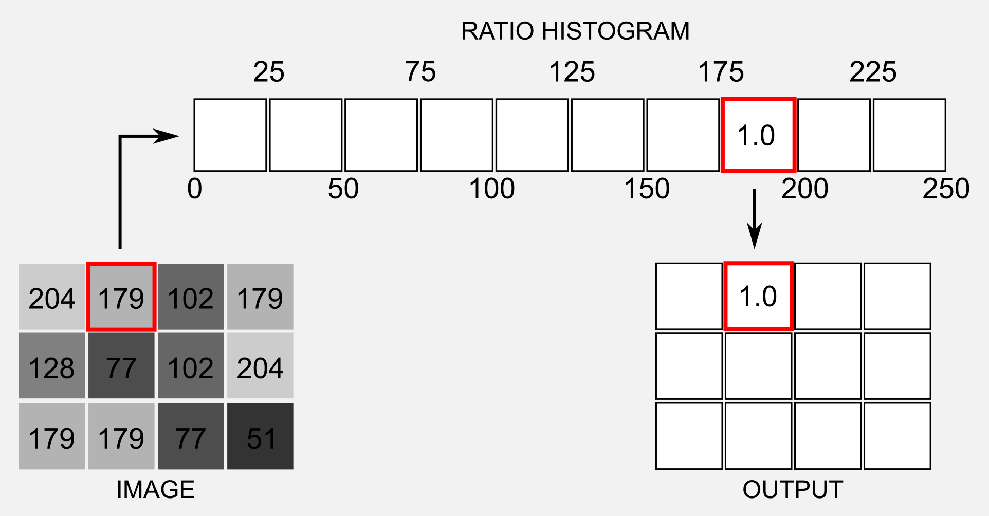
To simplify I took into account a single channel greyscale image and I considered the first (3x4) pixels on the top right corner. Each pixel has a value in the range [0,250]. Tthe pixel at the location (1,2) has a value of 179. We have to access the ratio histogram \(R\) and find the bin which corresponds to 179. Using a 10 bins histogram the position representing the value 179 is the number eight (bin [175, 200]). The value stored in this position (1.0) is taken and assigned to the location (1,2) of the output matrix, the image \(B\). This is the backprojection in a nutshell. Ok, it is time to write some code…

Implementation in python

Let’s start implementing the algorithm step-by-step in Numpy. The code below works with one dimensional histograms (greyscale image) but it can be easily extended to work with multi-dimensional histograms. For multidimensional histogram it is necessary to use the method numpy.histogramdd instead of the standard numpy.histogram. The name of the variables I am going to use is the same used by Swain and Ballard in their article. First of all we need a function to get the ratio histogram \(R\) given the model histogram \(M\) and the image histogram \(I\).

def return_ratio_histogram(M, I):
    ones_array = np.ones(I.shape)
    R = np.minimum(np.true_divide(M, I), ones_array)
    return R

The next step is the equivalent of the function \(h(c)\) which maps the pixel of the input image to the value of the ratio histogram \(R\). Here I supposed that the bins were equally spaced and that the highest pixel value was 255, however this is not always the case:

def return_backprojected_image(image, R):
    indexes = np.true_divide(image.flatten, 255)*R.shape[0]
    B = R.astype(int)[indexes]
    return B

We call B the image returned by the return_backprojected() method. In the next step we apply a circular convolution of radius r to the backrpojected image B. Numpy does not implement a 2D convolution operator we use the OpenCV method cv2.filter2D:

def convolve(B, r):
    D = cv2.getStructuringElement(cv2.MORPH_ELLIPSE,(r,r))
    cv2.filter2D(B, -1, D, B)
    B = np.uint8(B)
    cv2.normalize(B, B, 0, 255, cv2.NORM_MINMAX)
    return B

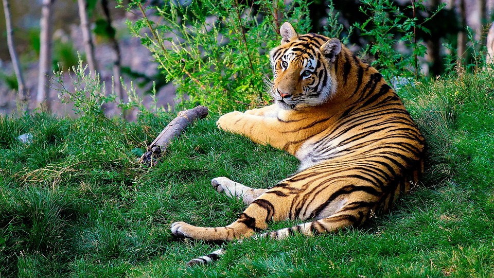
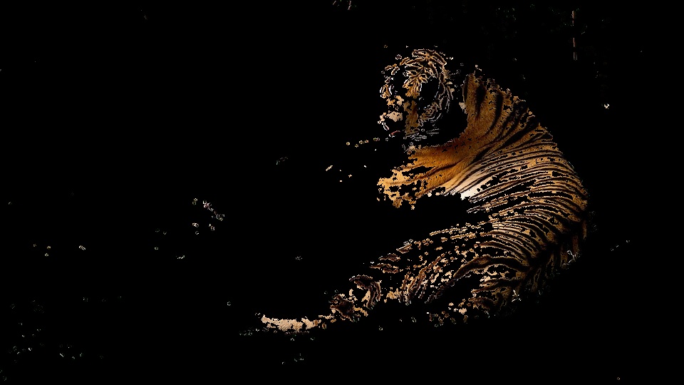
Implementing the algorithm from scratch is not necessary because OpenCV has an useful function called calcBackProject. I will use this function to isolate the tiger’s fur in the image below (which you can download here):

import cv2
import numpy as np

#Loading the image and converting to HSV
image = cv2.imread('tiger.jpg')
image_hsv = cv2.cvtColor(image,cv2.COLOR_BGR2HSV)

#I take a subframe of the original image
#corresponding to the fur of the tiger
model_hsv = image_hsv[225:275,625:675]

#Get the model histogram M and Normalise it
M = cv2.calcHist([model_hsv], channels=[0, 1], mask=None, 
                  histSize=[180, 256], ranges=[0, 180, 0, 256] )
M = cv2.normalize(M, alpha=0, beta=255, norm_type=cv2.NORM_MINMAX)

#Backprojection of our original image using the model histogram M
B = cv2.calcBackProject([image_hsv], channels=[0,1], hist=M, 
                         ranges=[0,180,0,256], scale=1)

#Now we can use the function convolve(B, r) we created previously
B = convolve(B, r=5)
 
#Threshold to clean the image and merging to three-channels
_, thresh = cv2.threshold(B, 50, 255, 0)
B_thresh = cv2.merge((thresh, thresh, thresh))

#Using B_tresh as a mask for a binary AND with the original image
cv2.imwrite('result.jpg', cv2.bitwise_and(image, B_thresh))

We can obtain better results applying the algorithm multiple times and using different models sampled from the object we want to find. I implemented a multi-backprojection version of the algorithm in deepgaze. The class is called MultiBackProjectionColorDetector and it can be initialised and used in a few lines. The main advantage of the deepgaze class is that you can pass a list of models and accumulate the results of each filter:

import cv2
from deepgaze.color_detection import MultiBackProjectionColorDetector

#Loading the main image
img = cv2.imread('tiger.jpg')

#Creating a python list and appending the model-templates
#In this case the list are preprocessed images but you
#can take subframes from the original image
template_list=list()
template_list.append(cv2.imread('model_1.jpg')) #Load the image
template_list.append(cv2.imread('model_2.jpg')) #Load the image
template_list.append(cv2.imread('model_3.jpg')) #Load the image
template_list.append(cv2.imread('model_4.jpg')) #Load the image
template_list.append(cv2.imread('model_5.jpg')) #Load the image

#Defining the deepgaze color detector object
my_back_detector = MultiBackProjectionColorDetector()
my_back_detector.setTemplateList(template_list) #Set the template

#Return the image filterd, it applies the backprojection,
#the convolution and the mask all at once
img_filtered = my_back_detector.returnFiltered(img, 
                                               morph_opening=True, blur=True, 
                                               kernel_size=3, iterations=2)
cv2.imwrite("result.jpg", img_filtered)

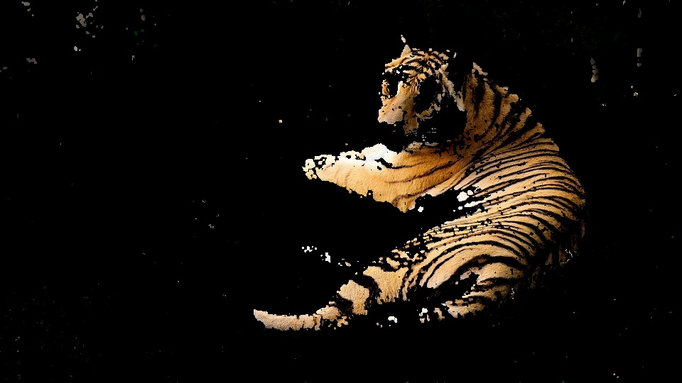
As you can see we got better results. Having multiple templates allows the model to have a more complete representation of the object. This approach can have some issues, having more templates means having more noise. In fact the amount of background noise captured in the second image is higher than the first one. An intelligent use of morphing operations can attenuate the problem, in this sense the choice of the kernel size is crucial. The full version of the code (and the five templates) is available on the deepgaze repository.

Google Chrome’s dinosaur game

We know the theory and how to implement the algorithm in python, it’s time for a real application. While I was writing this post I lost my internet connection (probably because Valerio Biscione was abusing the network). When you lost the connection and you are using Chrome a tiny dinosaur will appear. This 8-bit T-Rex can jump when you press UP and drop when you press DOWN. The goal of the game is to go on until death (in my case it happens quite soon). To play the game you don’t have to turn off your router, here you can find an online version. I recently saw an amazing video on youtube made by Ivan Seidel where the genetic algorithm has been used to evolve autonomous dinosaurs that can go ahead with an impressive accuracy. Recalling that video I came out with this idea: implementing an hand controller to play the Dinosaur game. Hand Up > Dino Up, Hand Down > Dino Down. In Linux it is possible to simulate the keyboard using the evdev event interface, which is part of the Linux kernel. In a few lines we can create our simulated keyboard and press KEY_UP and KEY_DOWN when we need it. For example, if you want to press KEY_DOWN for one second the minimalistic code to use is the following:

import time
from evdev import UInput, ecodes as e

ui = UInput()
ui.write(e.EV_KEY, e.KEY_DOWN, 1) #press the KEY_DOWN button
time.sleep(1)
ui.write(e.EV_KEY, e.KEY_DOWN, 0) #release the KEY_DOWN button

Remember that for security reason it is possible to use evdev only if you are superuser (run the script with sudo). I wrote the code using deepgaze and in particular the two classes MultiBackProjectionColorDetector and BinaryMaskAnalyser. Using the multi-backprojection I obtained the mask of my hand and with the method returnMaxAreaCenter() of the BinaryMaskAnalyser class I got the centre of the hand. When the centre is higher or lower than a predefined level the script executes a KEY_UP or a KEY_DOWN using evdev. This part should be very intuitive so I will not expand it further. You can watch the video on YouTube:

As you can see it is not so easy to control the dinosaur. Most of the time I was not able to anticipate the incoming cactus, but I am not good at this game also when I use the keyboard properly! If you want you can try, the full code is available on the deepgaze repository. Hopefully you will get an highest score…

References

Swain, M. J., & Ballard, D. H. (1991). Color indexing. International journal of computer vision, 7(1), 11-32.

Swain, M. J., & Ballard, D. H. (1992). Indexing via color histograms. In Active Perception and Robot Vision (pp. 261-273). Springer Berlin Heidelberg.