The Simplest Classifier: Histogram Comparison

Geometrical cues are the most reliable way to estimate objects identity. After all, we can recognise a chair also in a black and white image, we do not need colours or texture. However this is not always the case. In nature there are many examples where a colour identifies species, fruits and minerals. In our society distinctive colours are often used in trademark and logos. Think about Google and Facebook, the first is identified by a combination of blue, red, yellow and green, whereas the second is mainly blue.

Identifying objects only through colours can be considered crazy at first glance. However, also one of the most effective classifier the Convolutional Neural Network takes advantage of colours. Training the network on RGB images instead of greyscale ones, can make a huge difference. Moreover, our brain evolved to use colour. Colour helps the visual system to analyse complex images more efficiently, improving object recognition. Some psychological experiments showed how colour gives a strong contribution to memorisation and recognition (Wichmann and Sharpe, 2002). The histogram intersection algorithm uses the colour information to recognise objects. Let’s see how it works…

The histogram intersection algorithm

The histogram intersection algorithm was proposed by Swain and Ballard in their article “Color Indexing”. This algorithm is particular reliable when the colour is a strong predictor of the object identity. The histogram intersection does not require the accurate separation of the object from its background and it is robust to occluding objects in the foreground. An histogram is a graphical representation of the value distribution of a digital image. The value distribution is a way to represent the colour appearance and in the HVS model it represents the saturation of a colour. Histograms are invariant to translation and they change slowly under different view angles, scales and in presence of occlusions.

Now let’s give a mathematical foundation to the algorithm. Given the histogram \(I\) of the input image (camera frame) and the histogram \(M\) of the model (object frame), each one containing \(n\) bins, the intersection is defined as:

\[\sum_{j=1}^{n} min(I_{j}, M_{j})\]

The \(min\) function take as arguments two values and return the smallest one. The result of the intersection is the number of pixels from the model that have corresponding pixels of the same colours in the input image. To normalise the result between 0 and 1 we have to divide it by the number of pixels in the model histogram:

\[\frac{ \sum_{j=1}^{n} min(I_{j}, M_{j}) }{ \sum_{j=1}^{n} M_{j} }\]

That’s all. What we need is an histogram for each object we want to identify. When an unknown object image is given as input we compute the histogram intersection for all the stored models, the highest value is the best match.

Implementation in Python

In python we can easily play with histograms, for instance numpy has the function numpy.histogram() and OpenCV the function cv2.calcHist(). To plot an histogram we can use the matplotlib function matplotlib.pyplot.hist(). The main parameters to give as input to these functions are the array (or image), the number of bins and the lower and upper range of the bins. In OpenCV two histograms can be compared using the function cv2.compareHist() which take as input the histogram parameters and the comparison method. Among the possible methods there is also the CV_COMP_INTERSECT which is an implementation of the histogram intersection method. Numpy does not have a built-in function for comparing histograms, but we can implement it in a few lines. First of all we have to create two histograms:

mu_1 = -4 #mean of the first distribution
mu_2 = 4 #mean of the second distribution
data_1 = np.random.normal(mu_1, 2.0, 1000)
data_2 = np.random.normal(mu_2, 2.0, 1000)
hist_1, _ = np.histogram(data_1, bins=100, range=[-15, 15])
hist_2, _ = np.histogram(data_2, bins=100, range=[-15, 15])

The code below generates two histograms using values sampled from two different normal distribution (mean=mu_1, mu_2; std=2.0). The histograms have 100 bins which contains values in the range [-15, 15]. Once we have the two numpy histograms we can use the following function to compare them:

def return_intersection(hist_1, hist_2):
    minima = np.minimum(hist_1, hist_2)
    intersection = np.true_divide(np.sum(minima), np.sum(hist_2))
    return intersection

Plotting the histogram generated from \(\mathcal{N}(4, 2)\) and the one generated from \(\mathcal{N}(-4, 2)\) we can easily visualise the intersection:

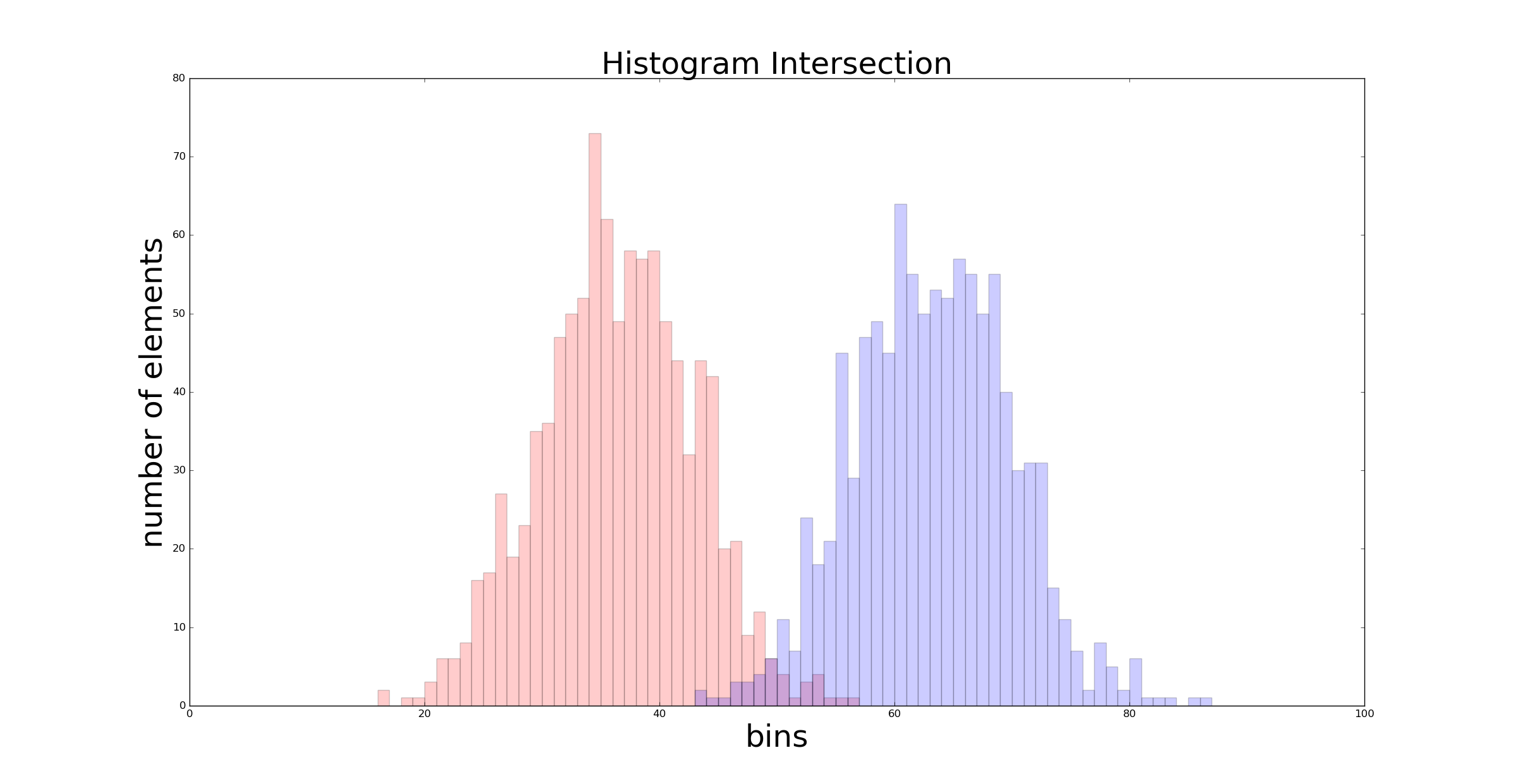
On the x axis there are the 100 bins, whereas on the y axis is represented the number of elements inside each bin. You can see the first bin as a counter for the elements comprised between [-15.0, -15.15), the second bin as a counter for the elements in the range [-15.15, -15.30), and so on. The intersection between the red graph and the blue one is what we are looking for. That intersection is larger when the two distribution are similar. In the previous example the intersection value returned by return_intersection() was 0.035. If we choose normal distributions with closest mean \(\mathcal{N}(2, 2)\) and \(\mathcal{N}(-2, 2)\) we get a larger intersection:

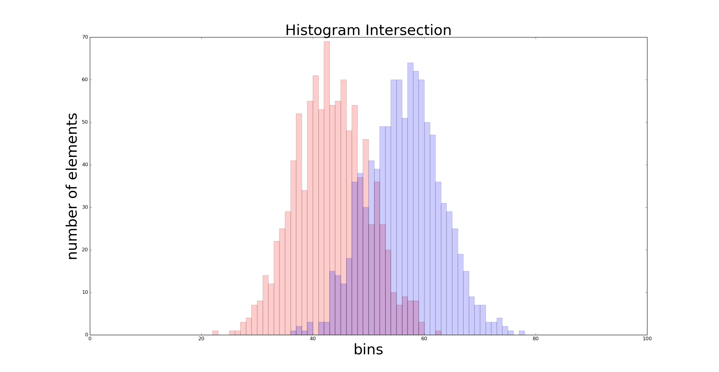
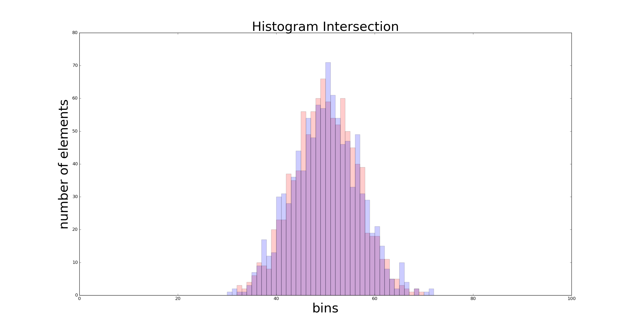
The new intersection value is 0.329. In the extreme case of distributions with the same mean and standard deviation \(\mathcal{N}(0, 2)\) we get an intersection value which is close to 1 (in this case it is 0.89), as shown in the following graph :

In the next section we are no more dealing with histograms because I have implemented a full version of the algorithm in deepgaze. I suggest you to clone the repository since it includes the full working example and some pre-processed images to play with. In deepgaze it is extremely easy to initialise a histogram classifier and use it. Let’s see a practical example…

Superheroes classification

Maybe you already noticed that each superheroes from the Marvel and DC universe has a distinctive multicolour fingertip. In the image below you can visually get the differences:

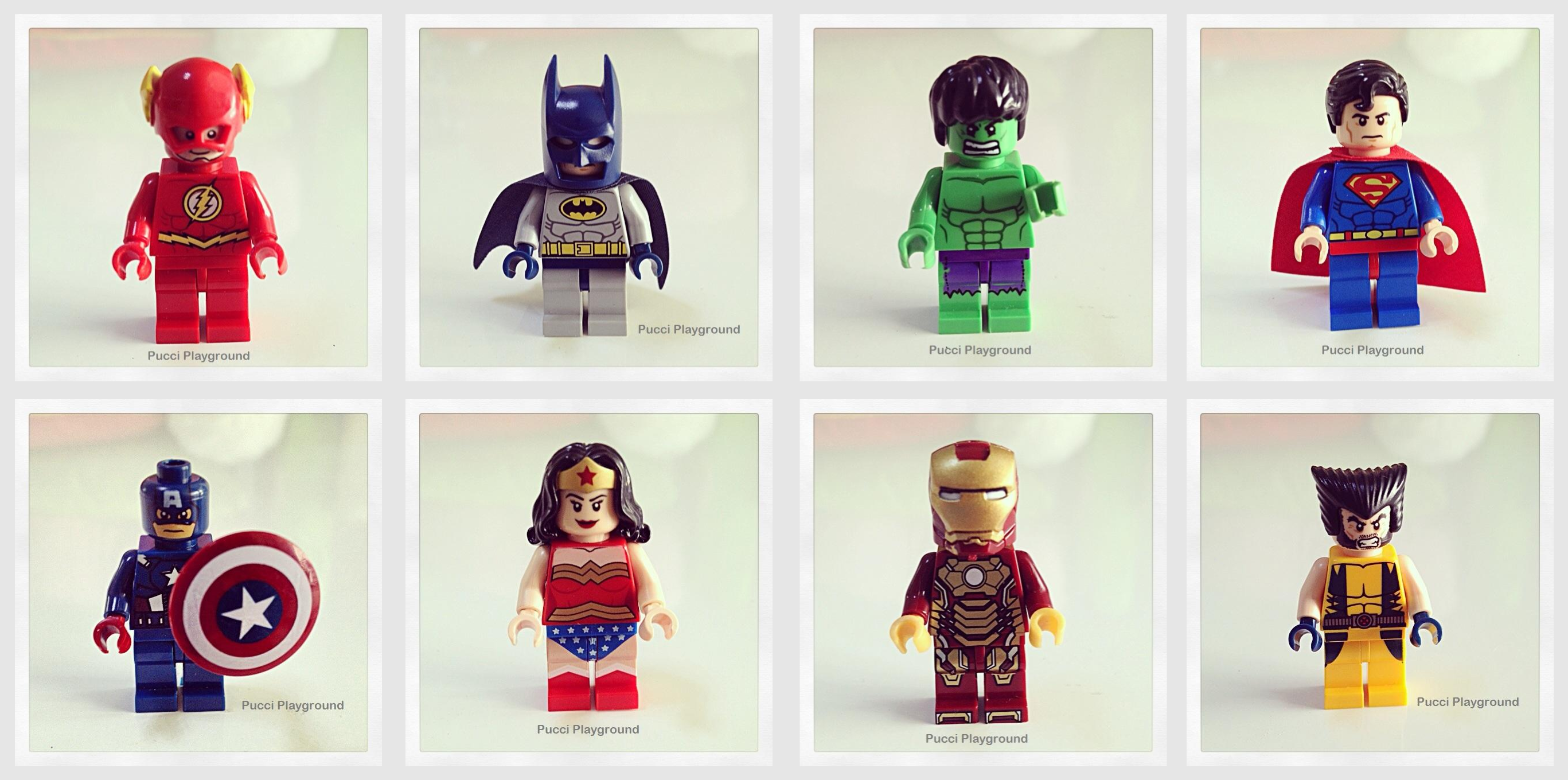
In this example I will use the deepgaze colour classifier to recognise eight superheroes. First of all we have to import some libraries and the deepgaze module, then we can initialise the classifier object calling HistogramColorClassifier(). As parameter we can give the number of channel (in a RGB image there are three channels) then the number of bins for each channel and the range of the values inside each bin.:

import cv2
import numpy as np
from deepgaze.color_classification import HistogramColorClassifier

my_classifier = HistogramColorClassifier(channels=[0, 1, 2], 
                                         hist_size=[128, 128, 128], 
                                         hist_range=[0, 256, 0, 256, 0, 256], 
                                         hist_type='BGR')

Now we have to load the models. You can read the image with the OpenCV function cv2.imread() and then load it calling the deepgaze addModelHistogram() function. You have to repeat this operation for all the models you want to store in the classifier. In my case I stored eight model in the following order [Flash, Batman, Hulk, Superman, Capt. America, Wonder Woman, Iron Man, Wolverine]. For each model I called the addModelHistogram() function as follow:

model_1 = cv2.imread('model_1.png') #Flash Model
my_classifier.addModelHistogram(model_1)

model_2 = cv2.imread('model_2.png') #Batman Model
my_classifier.addModelHistogram(model_2)

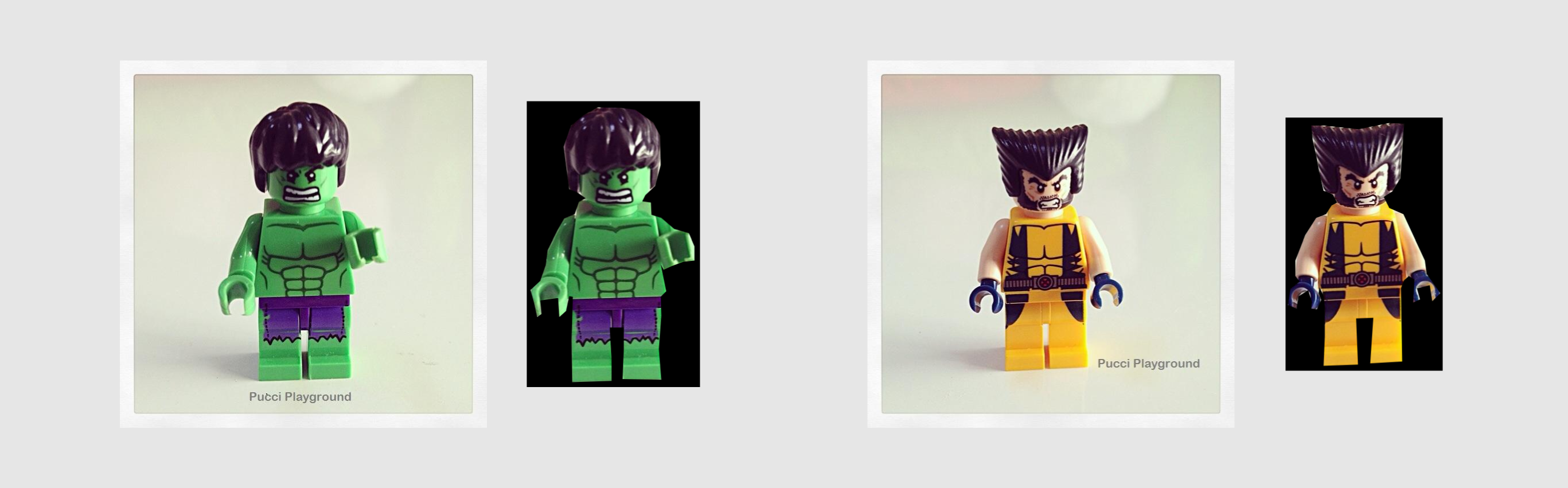
In the article “Color Indexing” the authors recommend to crop the model from the background. This operation can be annoying but you can obtain good result with a gross cropping. In the deepgaze repository you can find 10 different images cropped and ready to use. Each model was taken from a frontal image of the puppet and manually cropped to isolate the foreground from the background:

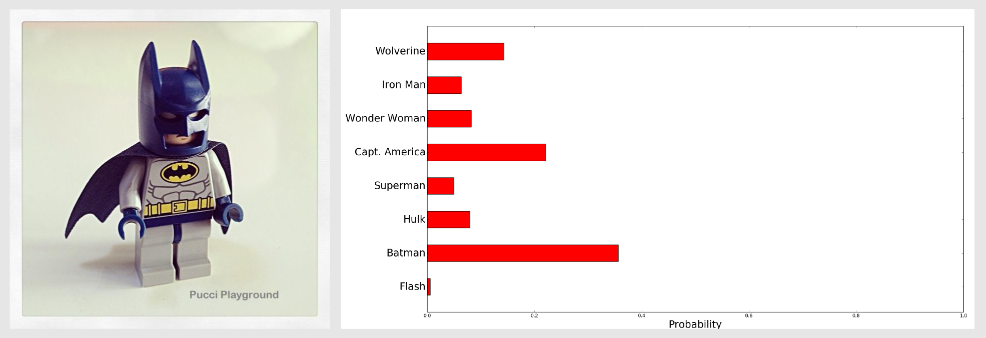
It is time to test the classifier. For the first trial I used an image of Batman. After loading the image with OpenCV I compared it with the models using a single call to returnHistogramComparisonArray() as follow:

image = cv2.imread('image_2.jpg') #Batman Test
comparison_array = my_classifier.returnHistogramComparisonArray(image, 
                                                                method="intersection")

The method returnHistogramComparisonArray() returns a numpy array which contains the result of the intersection between the image and the models. In this function it is possible to specify the comparison method, intersection refers to the method we discussed in this article. Other available methods are correlation (Pearson Correlation Coefficient), chisqr (Chi-Square) and bhattacharyya which is an implementation of the Bhattacharyya distance measure. The following table shows the distance value returned by each method in case of exact match, half match and mismatch of the two histograms:

HISTOGRAMS	CORRELATION	CHI SQUARE	INTERSECTION	BHATTACHARYYA
Exact Match	1.0	0.0	1.0	0.0
Half Match	0.7	0.67	0.5	0.55
Mismatch	-1.0	2.0	0.0	1.0

To check the result of the comparison we can print the values stored in the comparison_array:

0.00818883 #Flash
0.55411926 #Batman
0.12405966 #Hulk
0.07735263 #Superman
0.34388389 #Capt. America
0.12672027 #Wonder Woman
0.09870308 #Iron Man
0.2225694  #Wolverine

As you can see the second value (~0.55) is the highest one, meaning that the second model (Batman) has the best match with the input image. This value is the raw distance, to obtain a probability distribution we have to normalise the array dividing it by the sum of the values:

probability_array = comparison_array / np.sum(comparison_array)

The result of this operation is a new vector which values sum up to 1:

0.00526411 #Flash
0.35621003 #Batman
0.07975051 #Hulk
0.04972536 #Superman
0.22106232 #Capt. America
0.08146086 #Wonder Woman
0.06345029 #Iron Man
0.14307651 #Wolverine

Now we can say that the second model has a probability of 35.6% of being the correct match:

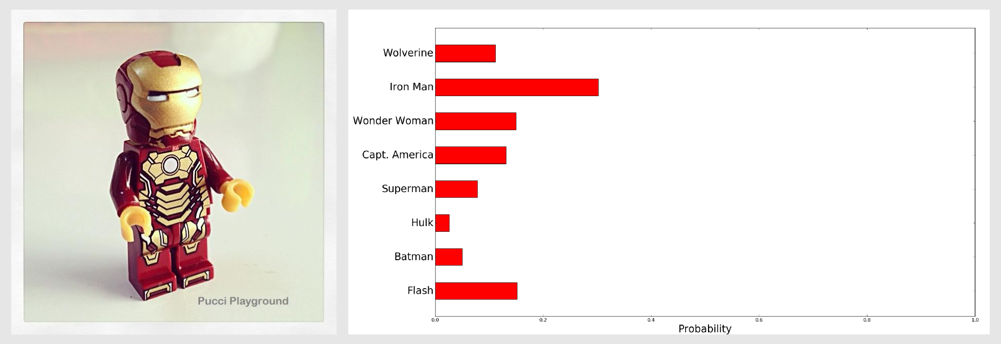
With Batman was easy to get an high confidence value because Batman’s multicolor fingerprint is pretty distinctive. Let’s test the classifier on something more complicated. I gave as model a frontal image of Ironman with the helmet on. For the test I used an image where Ironman was turned on the right and did not have the helmet. I called the returnHistogramComparisonArray() and normalised the output, then with matplotlib I generated a bar chart:

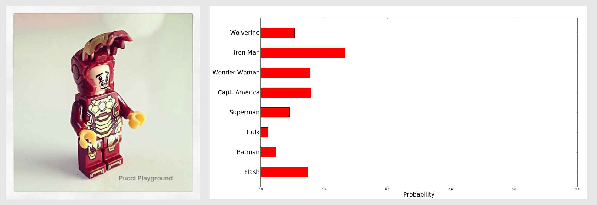
Also in this case we got a good result (26.6%). What happens if the image is in a different position and there are some additional colours respect to the model? We can try with Wonder Woman:

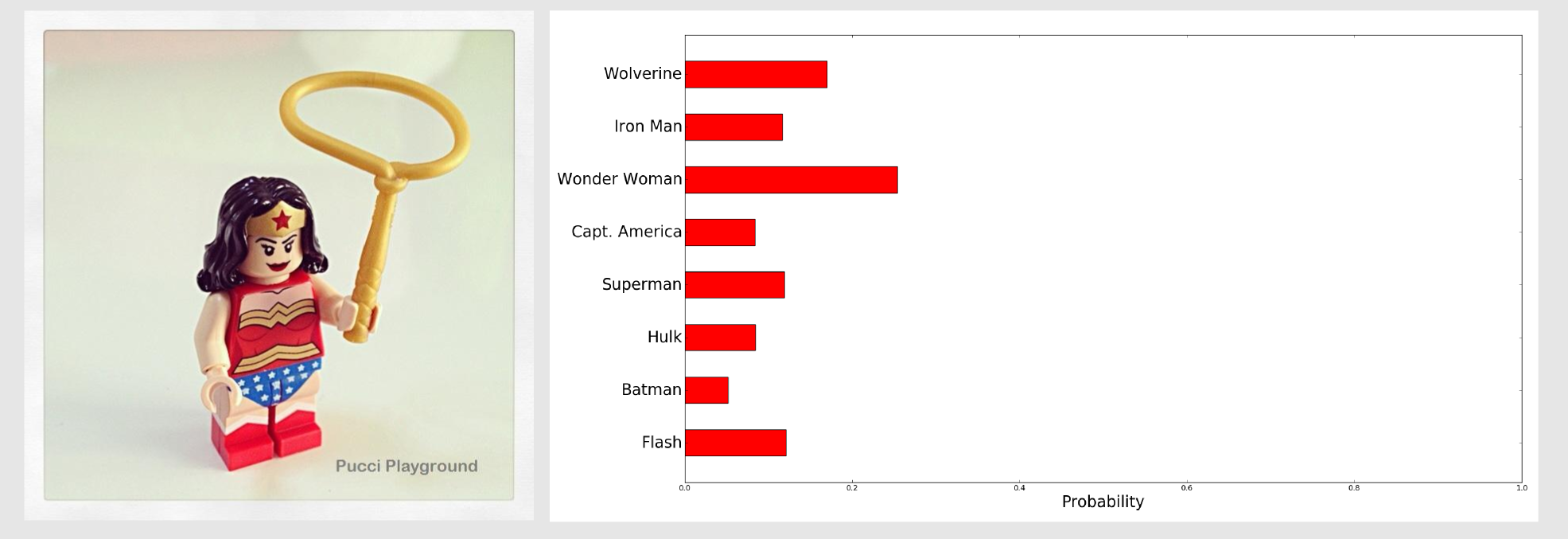
We got a confidence of 25.4% which was enough to identify the puppet. As we said the histogram intersection is reliable when there are small change in the object perspective and when there is noise in the background. If you want you can test the other images downloading the example from the deepgaze repository. For all the images the highest value identified the correct superhero. In their article Swain and Ballard tested the histogram intersection on a dataset containing 66 models. For the 66-object dataset the correct model was the best matches 29 of 32 times and in the other 3 cases the correct model was the second highest match. If you have the occasion to test the model with larger datasets please share your results in the comments below.

Acknowledgments

The superheroes images are courtesy of Christopher Chong.

References

Swain, M. J., & Ballard, D. H. (1991). Color indexing. International journal of computer vision, 7(1), 11-32.

Swain, M. J., & Ballard, D. H. (1992). Indexing via color histograms. In Active Perception and Robot Vision (pp. 261-273). Springer Berlin Heidelberg.

Wichmann, F. A., Sharpe, L. T., & Gegenfurtner, K. R. (2002). The contributions of color to recognition memory for natural scenes. Journal of Experimental Psychology: Learning, Memory, and Cognition, 28(3), 509.