An overview of Gaussian Mixture Models
In this post I will provide an overview of Gaussian Mixture Models (GMMs), including Python code with a compact implementation of GMMs and an application on a toy dataset. The post is based on Chapter 11 of the book “Mathematics for Machine Learning” by Deisenroth, Faisal, and Ong available in PDF here and in the paperback version here.

What do you need to know? In order to enjoy the post you need to know some basic probability theory (random variables, probability distributions, etc), some calculus (derivatives), and some Python if you want to delve into the programming part. The post follows this plot:
- A quick recap on Gaussian distributions
- Likelihood and Maximum Likelihood (ML) of a Gaussian
- Example: fitting a distribution with a Gaussian
- Intro to latent variable models
- Gaussian Mixture Models (GMMs)
- Likelihood of a GMM and Responsibilities
- Expectation Maximization (EM) for GMM
- Example: fitting a distribution with GMMs (with Python code)
- Pros and Cons of GMMs and EM
Where to find the code used in this post? Essential code is included in the post itself, whereas an extended version of the code is available in my repository. The dataset used in the examples is available as a lightweight CSV file in my repository, this can be easily copy-pasted in your local folder.
Quick recap on Gaussian distributions
Since we are going to extensively use Gaussian distributions I will present here a quick recap. A Gaussian distribution is a continuous probability distribution that is characterized by its symmetrical bell shape. A univariate Gaussian distribution is defined as follows:
\[p\left(x \mid \mu, \sigma^{2}\right)= \mathcal{N}\left(\mu, \sigma^{2}\right) = \frac{1}{\sqrt{2 \pi \sigma^{2}}} \exp \left(-\frac{(x-\mu)^{2}}{2 \sigma^{2}}\right).\]Note that \(\mu\) and \(\sigma\) are scalars representing the mean and standard deviation of the distribution. We like Gaussians because they have several nice properties, for instance marginals and conditionals of Gaussians are still Gaussians. Thanks to these properties Gaussian distributions have been widely used in a variety of algorithms and methods, such as the Kalman filter and Gaussian processes.
The univariate Gaussian defines a distribution over a single random variable, but in many problems we have multiple random variables thus we need a version of the Gaussian which is able to deal with this multivariate case. The multivariate Gaussian distribution can be defined as follows:
\[p(\boldsymbol{x} \mid \boldsymbol{\mu}, \boldsymbol{\Sigma}) = \mathcal{N}\left(\boldsymbol{\mu}, \boldsymbol{\Sigma}\right) = (2 \pi)^{-\frac{D}{2}}|\boldsymbol{\Sigma}|^{-\frac{1}{2}} \exp \left(-\frac{1}{2}(\boldsymbol{x}-\boldsymbol{\mu})^{\top} \boldsymbol{\Sigma}^{-1}(\boldsymbol{x}-\boldsymbol{\mu})\right).\]Note that \(\boldsymbol{\mu}\) and \(\boldsymbol{\Sigma}\) are not scalars but a vector (of means) and a matrix (of variances). The value \(|\boldsymbol{\Sigma}|\) is the determinant of \(\boldsymbol{\Sigma}\), and \(D\) is the number of dimensions \(\boldsymbol{x} \in \mathbb{R}^{D}\). Interpolating over \(\boldsymbol{\mu}\) has the effect of shifting the Gaussian on the \(D\)-dimensional (hyper)plane, whereas changing the matrix \(\boldsymbol{\Sigma}\) has the effect of changing the shape of the Gaussian.
Likelihood of a Gaussian
Let’s suppose we are given a bunch of data and we are interested in finding a distribution that fits this data. We can assume that the data has been generated by an underlying process, and that we want to model this process. We can choose a Gaussian distribution to model our data. The goal now is to find mean and variance of the Gaussian. This can be done via Maximum Likelihood (ML) estimation.
We want to estimate the mean \(\mu\) of a univariate Gaussian distribution (suppose the variance is known), given a dataset of points \(\mathcal{X}= \{x_{n} \}_{n=1}^{N}\). We can proceed as follows: (i) define the likelihood (predictive distribution of the training data given the parameters) \(p(\mathcal{X} \vert \mu)\), (ii) evaluate the log-likelihood \(\log p(\mathcal{X} \vert \mu)\), and (iii) find the derivative of the log-likelihood with respect to \(\mu\). We are under the assumption of independent and identically distributed (i.i.d.) random variables. The three steps are:
\[\begin{aligned} p(\mathcal{X} \vert \mu) &=\prod_{n=1}^{N} \frac{1}{\sqrt{2 \pi \sigma^{2}}} \exp -\frac{\left(x_{n}-\mu\right)^{2}}{2 \sigma^{2}}, \\ \mathcal{L} &= \log p(\mathcal{X} \vert \mu) =\sum_{n=1}^{N}\left[\log \left(\frac{1}{\sqrt{2 \pi \sigma^{2}}}\right)-\frac{\left(x_{n}-\mu\right)^{2}}{2 \sigma^{2}}\right], \\ \frac{d \mathcal{L}}{d \mu} &=\sum_{n=1}^{N} \frac{x_{n}-\mu}{\sigma^{2}}. \end{aligned}\]Note that applying the log to the likelihood in the second step, turned products into sums and helped us getting rid of the exponential. The third step has given us the derivative of the log-likelihood, what we need to do now is to set the derivative to zero and isolate the parameter of interest \(\mu\). This lead to the ML estimator for the mean of a univariate Gaussian:
\[\mu_{\text{ML}}=\frac{\sum_{n=1}^{N} x_{n}}{N}.\]The equation above just says that the ML estimate of the mean can be obtained by summing all the values then divide by the total number of points. The ML estimate of the variance can be calculated with a similar procedure, starting from the log-likelihood and differentiating with respect to \(\sigma\), then setting the derivative to zero and isolating the target variable:
\[\sigma_{\text{ML}}^{2}=\frac{\sum_{n=1}^{N} (x_{n} - \mu)^{2}}{N}.\]Example: fitting distributions
Fitting unimodal distributions. Let’s consider a simple example and let’s write some Python code for it. Suppose we have a set of data that has been generated by an underlying (unknown) distribution. For this example, I will consider the body measurements dataset provided by Heinz et al. (2003) that you can download from my repository. This is a lightweight CSV dataset, that you can simply copy and paste in your local text file. In particular, I will gather the subset of body weight (in kilograms). Once we have the data, we would like to estimate the mean and standard deviation of a Gaussian distribution by using ML. This can be easily done by plugging-in the closed-form expressions of mean and standard deviation:
import numpy as np

data = np.genfromtxt('./bdims.csv', delimiter=',', skip_header=1)[:,-3]
N = len(data)
mean = data.sum() / N
std = np.sqrt(np.sum((data - mean)**2) / N)
print("{mean:.3f} +- {std:.3f} (N={N:d})".format(mean=mean, std=std, N=N))
The snippet will print:
69.148 +- 13.333 (N=507)
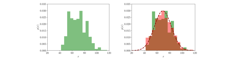
which seems to be a good approximation of the true underlying distribution give the 507 measurements. For the law of large numbers, as the number of measurements increases the estimation of the true underlying parameters gets more precise. We can assign the data points to an histogram of 15 bins (green) and visualize the raw distribution (left image). Then we can plot the Gaussian estimated via ML and draw 1000 samples from it, assigning the samples to the same 15 bins (red). The overlap between real data (green) and simulated data (red) shows how well our approximation fits the original data (right image):
Fitting multimodal distributions. We approximated the data with a single Gaussian distribution. However, looking at the overlap between the real data and the data sampled from our model we notice some discontinuities. It is likely that there are latent factors of variation that originated the data. For instance, we know that height is correlated with age, weight, and sex, therefore it is possible that there are sub-populations we did not capture using a single Gaussian model resulting in a poor fit. How can we solve this problem?
A latent variable approach
Recap: we have a dataset (body weight) that is likely to have been produced by multiple underlying sub-distributions.
Goal: we want to find a way to represent the presence of sub-populations within the overall population.
We can assume that each data point \(x_{n}\) has been produced by a latent variable \(z\) and express this causal relation as \(z \rightarrow x\). In our particular case, we can assume \(z\) to be a categorical distribution representing \(K\) underlying distributions. Each data point can be mapped to a specific distribution by considering \(z\) as a one-hot vector identifying the membership of that data point to a component. For instance, \(\boldsymbol{z}=\left[z_{1}, z_{2}, z_{3}\right]^{\top}=[0,1,0]^{\top}\) means that the data point belongs to the second component. This corresponds to a hard assignment of each point to its generative distribution. In reality, we do not have access to the one-hot vector, therefore we impose a distribution over \(z\) representing a soft assignment:
\[p(\boldsymbol{z})=\boldsymbol{\pi}=\left[\pi_{1}, \ldots, \pi_{K}\right]^{\top}, \quad \text{with} \quad 0 \leq \pi_{k} \leq 1 \quad \text{and} \quad \sum_{k=1}^{K} \pi_{k}=1.\]Now, each data point do not exclusively belong to a certain component, but to all of them with different probability. This approach defines what is known as mixture models.
Gaussian Mixture Models (GMMs)
Our goal is to find the underlying sub-distributions in our weight dataset and it seems that mixture models can help us. Here is an idea, what if we use multiple Gaussians as part of the mixture? Each Gaussian would have its own mean and variance and we could mix them by adjusting the proportional coefficients \(\pi\). This would be like mixing different sounds by using the sliders on a console. Something like this is known as a Gaussian Mixture Model (GMM).
Deriving the likelihood of a GMM from our latent model framework is straightforward. We first collect the parameters of the Gaussians into a vector \(\boldsymbol{\theta}\). The likelihood \(p(x \vert \boldsymbol{\theta})\) is obtained through the marginalization of the latent variable \(z\) (see Chapter 8 of the book). In our case, marginalization consists of summing out all the latent variables from the joint distribution \(p(x, z)\) which yelds
\[p(x \mid \boldsymbol{\theta})=\sum_{z} p(x \mid \boldsymbol{\theta}, z) p(z \mid \boldsymbol{\theta})\]We can now link this marginalization to the GMM by recalling that \(p(x \mid \boldsymbol{\theta}, z_{k})\) is a Gaussian distribution \(\mathcal{N}\left(x \mid \mu_{k}, \sigma_{k}\right)\) with \(z\) consistsing of \(K\) components. A specific weight \(\pi_{k}\) represents the probability of the \(k\)-th component \(p(z_{k}=1 \vert \boldsymbol{\theta})\). It follows that a GMM with \(K\) univariate Gaussian components can be defined as
\[\mathcal{N}\left(\mu_{k}, \sigma_{k} \right) = \sum_{k=1}^{K} \pi_{k} \mathcal{N}\left(x \mid \mu_{k}, \sigma_{k}\right) \quad \text{where}\] \[0 \leqslant \pi_{k} \leqslant 1, \quad \sum_{k=1}^{K} \pi_{k}=1 \quad \text{and} \quad \boldsymbol{\theta}=\left\{\mu_{k}, \sigma_{k}, \pi_{k} \right\}_{k=1}^{K}\]Similarly we can define a GMM for the multivariate case:
\[\mathcal{N}\left(\boldsymbol{\mu}_{k}, \boldsymbol{\Sigma}_{k} \right) = \sum_{k=1}^{K} \pi_{k} \mathcal{N}\left(\boldsymbol{x} \mid \boldsymbol{\mu}_{k}, \boldsymbol{\Sigma}_{k}\right)\]under identical constraints for \(\pi\) and with \(\boldsymbol{\theta}=\left\{\boldsymbol{\mu}_{k}, \boldsymbol{\Sigma}_{k}, \pi_{k} \right\}_{k=1}^{K}\). GMMs are more expressive than simple Gaussians and they are often able to capture subtle differences in the data.
Sampling from a GMM: it is possible to sample new data points from our GMM by ancestral sampling. We start by sampling a value from the parent distribution, that is categorical, and then we sample a value from the Gaussian associated with the categorical index. In our latent variable model this consists of sampling a mixture component according to the weights \(\boldsymbol{\pi}=\left[\pi_{1}, \ldots, \pi_{K}\right]^{\top}\), then we draw a sample from the corresponding Gaussian distribution.
Posterior distribution of a GMM: we would like to know what is the probability that a certain data point has been generated by the \(k\)-th component that is, we would like to estimate the posterior distribution
\[p\left(z_{k}=1 \mid x\right)=\frac{p\left(z_{k}=1\right) p\left(x \mid z_{k}=1\right)}{p(x)}.\]Note that \(p(x)\) is just the marginal we have estimated above and \(p(z_{k}=1) = \pi_{k}\). Therefore, we have all we need to get the posterior
\[p\left(z_{k}=1 \mid x\right)=\frac{p\left(z_{k}=1\right) p\left(x \mid z_{k}=1\right)}{\sum_{j=1}^{K} p\left(z_{j}=1\right) p\left(x \mid z_{j}=1\right)}=\frac{\pi_{k} \mathcal{N}\left(x \mid \mu_{k}, \sigma_{k}\right)}{\sum_{j=1}^{K} \pi_{j} \mathcal{N}\left(x \mid \mu_{j}, \sigma_{j}\right)}.\]Important: GMMs are the weighted sum of Gaussian densities. This is different from the weighted sum of Gaussian random variables. For instance, given two Gaussian random variables \(\boldsymbol{x}\) and \(\boldsymbol{y}\), their weighted sum is defined as
\[p(a \boldsymbol{x}+b \boldsymbol{y})=\mathcal{N}\left(a \boldsymbol{\mu}_{x}+b \boldsymbol{\mu}_{y}, a^{2} \boldsymbol{\Sigma}_{x}+b^{2} \boldsymbol{\Sigma}_{y}\right).\]Likelihood of a GMM
In the following, I detail how to obtain a maximum likelihood estimate of a univariate GMM with \(K\) components. In doing so we have to follow the same procedure adopted for estimating the mean of the univariate Gaussian, which is done in three steps: (i) define the likelihood, (ii) estimate the log-likelihood, (iii) find the partial derivative of the log-likelihood with respect to \(\mu_{k}\). In short:
\[\begin{aligned} p(\mathcal{X} \mid \theta) &= \prod_{n=1}^{N} \sum_{k=1}^{K} \pi_{k} \frac{1}{\sqrt{2 \pi \sigma_{k}^{2}}} \exp -\frac{\left(x_{n}-\mu_{k} \right)^{2}}{2 \sigma_{k}^{2}}, \\ \mathcal{L} &= \log p(\mathcal{X} \mid \theta) = \sum_{n=1}^{N} \log \Bigg[ \sum_{k=1}^{K} \pi_{k} \frac{1}{\sqrt{2 \pi \sigma^{2}}} \exp -\frac{\left(x_{n}-\mu_{k}\right)^{2}}{2 \sigma_{k}^{2}} \Bigg], \\ \frac{\partial \mathcal{L}}{\partial \mu_{k}} &= \sum_{n=1}^{N} \frac{\pi_{k} \mathcal{N}\left(x_{n} \mid \mu_{k}, \sigma_{k}\right)}{\sum_{j=1}^{K} \pi_{j} \mathcal{N}\left(x_{n} \mid \mu_{j}, \sigma_{j}\right)} \cdot \frac{x_{n}-\mu_{k}}{\sigma_{k}^{2}}. \\ \end{aligned}\]If you compare the equations above with the equations of the univariate Gaussian you will notice that in the second step there is an an additional factor: the summation over the \(K\) components. This summation is problematic since it prevents the log function from being applied to the normal densities. Unlike the log of a product, the log of a sum does not immediately simplify. As a result the partial derivative of \(\mu_{k}\) depends on the \(K\) means, variances, and mixture weights.
Unidentifiability of the parameters. We can fit a single Gaussian on a dataset \(\mathcal{X}\) in one step using the ML estimator. This is possible because the posterior over the parameters \(p(\boldsymbol{\theta} \vert \mathcal{X})\) is unimodal that is, there is just one possible configuration of the parameters able to fit the data, let’s say \(\mu=a\) (suppose variance is given). In a GMM the posterior may have multiple modes. For instance, if you consider a GMM with two components, then there may be two possible optimal configurations, one at \(\mu_{1}=a, \mu_{2}=b\) and one at \(\mu_{1}=b, \mu_{2}=a\). We say that the parameters are not identifiable since there is not a unique ML estimation. Because of this issue the log-likelihood is neither convex nor concave, and has local optima. For additional details see Murphy (2012, Chapter 11.3, “Parameter estimation for mixture models”).
Responsibilities
How can we find the parameters of a GMM if we do not have a unique ML estimator? To answer this question, we need to introduce the concept of responsibility. It is possible to immediately catch what responsibilities are, if we compare the derivative with respect to \(\mu\) of the simple univariate Gaussian \(d \mathcal{L} / d \mu\), and the partial derivative of \(\mu_{k}\) of the univariate GMM \(\partial \mathcal{L} / \partial \mu_{k}\), given by
\[\frac{d \mathcal{L}}{d \mu} = \sum_{n=1}^{N} \frac{x_{n}-\mu}{\sigma^{2}}, \quad \text{and} \quad \frac{\partial \mathcal{L}}{\partial \mu_{k}} = \sum_{n=1}^{N} \underbrace{ \frac{\pi_{k} \mathcal{N}\left(x_{n} \mid \mu_{k}, \sigma_{k}\right)}{\sum_{j=1}^{K} \pi_{j} \mathcal{N}\left(x_{n} \mid \mu_{j}, \sigma_{j}\right)} } _{\text{responsibilities}} \cdot \frac{x_{n}-\mu_{k}}{\sigma_{k}^{2}}.\]As you can see the two terms are almost identical. The additional factor in the GMM derivative is what we call responsibilities. More formally, the responsibility \(r_{nk}\) for the \(k\)-th component and the \(n\)-th data point is defined as:
\[r_{nk} = p\left(z_{k}=1 \mid x_{n} \right) = \frac{\pi_{k} \mathcal{N}\left(x_{n} \mid \mu_{k}, \sigma_{k}\right)}{\sum_{j=1}^{K} \pi_{j} \mathcal{N}\left(x_{n} \mid \mu_{j}, \sigma_{j}\right)}.\]Now, if you have been careful you should have noticed that \(r_{nk}\) is just the posterior distribution we have estimated before. Exactly, the responsibility \(r_{nk}\) corresponds to \(p(z_{k}=1 \mid x_{n})\): the probability that the data point \(x_{n}\) has been generated by the \(k\)-th component of the mixture.
Note that \(r_{nk} \propto \pi_{k} \mathcal{N}\left(x_{n} \mid \mu_{k}, \sigma_{k}\right)\), meaning that the \(k\)-th mixture component has a high responsibility for a data point \(x_{n}\) when the data point is a plausible sample from that component. Note also that \(r_{n}:=\left[r_{n 1}, \ldots, r_{n K}\right]^{\top} \in \mathbb{R}^{K}\) is a probability vector since the individual responsibilities sum up to 1 due to the constraint on \(\pi\). You can consider this vector as a weighted assignment of a point to the \(K\) components. Responsibilities can be arranged in a matrix \(\in \mathbb{R}^{N \times K}\). The total responsibility of the \(k\)-th mixture component for the entire dataset is defined as
\[N_{k} = \sum_{n=1}^{N} r_{n k}.\]You can think of responsibilities as soft labels. Basically they are telling us from which Gaussian each data point is more likely to come from. If you have two Gaussians and the data point \(x_{1}\), then the associated responsibilities could be something like \(\{0.2, 0.8\}\) that is, there are \(20\%\) chances \(x_{1}\) comes from the first Gaussian and \(80\%\) chances it comes from the second Gaussian. Responsibilities impose a set of interlocking equations over means, (co)variances, and mixture weights, with the solution to the parameters requiring the values of the responsibilities (and vice versa).
A chicken-and-egg problem
To better understand what’s the main issue in fitting a GMM, consider this example. Suppose we have a dataset of real values \(\mathcal{X} = \{x_{1}, x_{2}, \dots, x_{N} \}\) and that half of the values has been generated by a Gaussian distribution \(\mathcal{N}_{A}\) while the other half from a Gaussian distribution \(\mathcal{N}_{B}\).
Goal: we want to know the parameters of the two Gaussians (mean and standard deviation), and from which Gaussian each data point comes from.
Given this setup, there are two possible scenarios:
- Unlabeled data, known parameters. In the first scenario, we are given the two Gaussians \(\mathcal{N}_{A}(\mu_A, \sigma_A)\) and \(\mathcal{N}_{B}(\mu_B, \sigma_B)\), but we do not know which Gaussian has generated the single data point (unlabeled data). Using the probability density function of each Gaussian we can estimate from which one each sample is more likely to come from (responsibilities).
- Labeled data, unknown parameters. In the second scenario, we know from which Gaussian each data point comes from \(x_{1} \sim \mathcal{N}_{A}, x_{2} \sim \mathcal{N}_{B}, x_{3} \sim \mathcal{N}_{A}, \dots\) We do not know the parameters of the Gaussians but we can find them by ML estimation over the two sets of data.
Now consider a third scenario that is unlabeled data, unknown parameters. How can we deal with this case? Well, this is problematic. To find the parameters of the distributions we need labeled data, and to label the data we need the parameters of the distribution. We have a chicken-and-egg problem.
However, the conceptual separation in two scenarios suggests an iterative methods. We could initialize two Gaussians with random parameters then iterate between two steps: (i) estimate the labels while keeping the parameters fixed (first scenario), and (ii) update the parameters while keeping the label fixed (second scenario). Iterating over these two steps will eventually reach a local optimum. It turns out that the solution we have just found is a particular instance of the Expectation Maximization algorithm.
Expectation Maximization (EM) for GMMs
The Expectation Maximization (EM) algorithm has been proposed by Dempster et al. (1977) as an iterative method for finding the maximum likelihood (or maximum a posteriori, MAP) estimates of a set of parameters. The algorithm consists of two step: the E-step in which a function for the expectation of the log-likelihood is computed based on the current parameters, and an M-step where the parameters found in the first step are maximized. Every EM iteration increases the log-likelihood function (or decreases the negative log-likelihood). For convergence, we can check the log-likelihood and stop the algorithm when a certain threshold \(\epsilon\) is reached, or alternatively when a predefined number of steps is reached.
The algorithm can be summarized in four steps:
Step 1 (Init): initialize the parameters \(\mu_k, \pi_k, \sigma_k\) to random values. This is not so trivial as it may seem. We must be careful in this very first step, since the EM algorithm will likely converge to a local optimum. We can initialize the components such that they are not too far from the data manifold, in this way we can minimize the risk they get stuck over outliers.
Step 2 (E-step): using current values of \(\mu_k, \pi_k, \sigma_k\) evaluate responsibilities \(r_{nk}\) (posterior distribution) for each component and data point
\[r_{nk} = \frac{\pi_{k} \mathcal{N}\left(x_{n} \mid \mu_{k}, \sigma_{k}\right)}{\sum_{j=1}^{K} \pi_{j} \mathcal{N}\left(x_{n} \mid \mu_{j}, \sigma_{j}\right)}.\]Step 3 (M-step): using responsibilities found in 2 evaluate new \(\mu_k, \pi_k\), and \(\sigma_k\). Using both the responsibilities and the \(N_{k}\) notation defined in the previous section, we can express in a compact way these equations for the univariate case:
\[\mu_{k} =\frac{1}{N_{k}} \sum_{n=1}^{N} r_{n k} x_{n}, \quad \sigma_{k} =\frac{1}{N_{k}} \sum_{n=1}^{N} r_{n k}\left(x_{n}-\mu_{k}\right)^{2}, \quad \pi_{k} =\frac{N_{k}}{N},\]and similarly the equations for \(\boldsymbol{\mu}_{k}\), \(\boldsymbol{\Sigma}_{k}\), and \(\pi_{k}\) in the multivariate case:
\[\boldsymbol{\mu}_{k} =\frac{1}{N_{k}} \sum_{n=1}^{N} r_{n k} \boldsymbol{x}_{n}, \quad \boldsymbol{\Sigma}_{k} =\frac{1}{N_{k}} \sum_{n=1}^{N} r_{n k}\left(\boldsymbol{x}_{n}-\boldsymbol{\mu}_{k}\right)\left(\boldsymbol{x}_{n}-\boldsymbol{\mu}_{k}\right)^{\top}, \quad \pi_{k} =\frac{N_{k}}{N}.\]Step 4 (Check): in this step we just check if the stopping criterium has been reached. This can be defined as reaching a certain number of iterations, or the moment the likelihood reaches a certain threshold. A validation set could also be used. If we go for the second solution we need to evaluate the negative log-likelihood and compare it against a threshold value \(\epsilon\)
\[-\sum_{n=1}^{N}\left[\log \left(\frac{1}{\sqrt{2 \pi \sigma^{2}}}\right)-\frac{\left(x_{n}-\mu\right)^{2}}{2 \sigma^{2}}\right] < \epsilon\]If this inequality evaluates to True then we stop the algorithm, otherwise we repeat from step 2. An interesting property of EM is that during the iterative maximization procedure, the value of the log-likelihood will continue to increase after each iteration (or likewise the negative log-likelihood will continue to decrease). In other words, the EM algorithm never makes things worse. Therefore, we can easily find a bug in our code if we see oscillations in the log-likelihood.
Example: fitting distributions by GMMs
We can now revisit the curve fitting example and apply a GMM made of univariate Gaussians. I have tried to keep the code as compact as possible and I added some comments to divide it in blocks based on the four steps described above. The extended version of the code (with plots) can be downloaded from my repository.
Changing the value of K you can change the number of components in the GMM. In the initialization step I draw the values of the mean from a uniform distribution with bounds defined as (approximately) one standard deviation on the data mean. I used a similar procedure for initializing the variances. As stopping criterium I used the number of iterations.
import numpy as np
from scipy.stats import norm

data = np.genfromtxt('./bdims.csv', delimiter=',', skip_header=1)
data = data[:,-3] # select the "weight" column in the dataset
N = data.shape[0] # number of data points
K=2 # two components GMM
tot_iterations = 100 # stopping criterium

# Step-1 (Init)
mu = np.random.uniform(low=42.0, high=95.0, size=K) # mean
sigma = np.random.uniform(low=5.0, high=10.0, size=K) # standard deviaiton
pi = np.ones(K) * (1.0/K) # mixing coefficients
r = np.zeros([K,N]) # responsibilities
nll_list = list() # used to store the neg log-likelihood (nll)

for iteration in range(tot_iterations):
    # Step-2 (E-Step)
    for k in range(K):
        r[k,:] = pi[k] * norm.pdf(x=data, loc=mu[k], scale=sigma[k])
    r = r / np.sum(r, axis=0) #[K,N] -> [N]

    # Step-3 (M-Step)
    N_k = np.sum(r, axis=1) #[K,N] -> [K]
    for k in range(K):
        mu[k] = np.sum(r[k,:] * data) / N_k[k] # update mean
        numerator = r[k] * (data - mu[k])**2
        sigma[k] = np.sqrt(np.sum(numerator) / N_k[k]) # update std
    pi = N_k/N # update mixing coefficient

    # Estimate likelihood and print info
    likelihood = 0.0
    for k in range(K):
        likelihood += pi[k] * norm.pdf(x=data, loc=mu[k], scale=sigma[k])
    nll_list.append(-np.sum(np.log(likelihood)))
    print("Iteration: "+str(iteration)+"; NLL: "+str(nll_list[-1]))
    print("Mean "+str(mu)+"\nStd "+ str(sigma)+"\nWeights "+ str(pi)+"\n")

    # Step-4 (Check)
    if(iteration==tot_iterations-1): break
Running the snippet will print various info on the terminal. Depending from the initialization values you can get different numbers, but when using K=2 with tot_iterations=100 the GMM will converge to similar solutions. In particular, most of the runs will converge to one Gaussian having mean \(\sim 55\) and the other \(\sim 75\), with the latter being wider than the former.
Iteration: 0; NLL: 2023.9831239837204
Mean [62.62522015 85.42117302]
Std [8.66814056 7.92670882]
Weights [0.71388279 0.28611721]
...
Iteration: 99; NLL: 2012.8920961962986
Mean [56.87072309 75.33979836]
Std [ 5.94313559 11.62910854]
Weights [0.33527742 0.66472258]
In the image below I have plotted the negative log-likelihood (left), a GMM with \(K=2\) (center), and a GMM with \(K=5\) (right). The data of the original dataset have been mapped into 15 bins (green), and 1000 samples from the GMM have been mapped to the same bins (red).
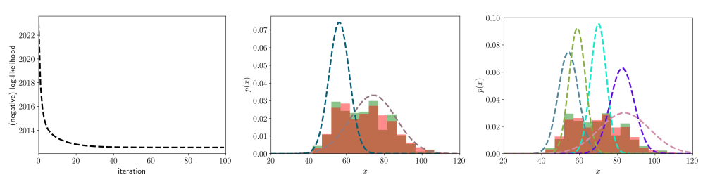
As you can see the negative log-likelihood rapidly goes down in the first iterations without anomalies. We can look at the overlap between the original data (green) and the samples from the GMM (red) to verify how close the two distributions are. The GMM with two components is doing a good job at approximating the distribution, but adding more components seems to be even better. However, we cannot add components indefinitely because we risk to overfit the training data (a validation set can be used to avoid this issue).
Pros and Cons
Pros:
- GMMs are easy to implement and can be used to model both univariate and multivariate distributions.
- EM is guaranteed to converge to a minimum (most of the time local) and the log-likelihood is guaranteed to decrease at each iteration (good for debug).
- EM is faster and more stable than other solutions (e.g. gradient descent).
- EM makes it easy to deal with constraints (e.g. positive definiteness of the covariance matrix in multivariate components).
Cons:
- Parameter initialization (step 1) is delicate and prone to collapsed solutions (e.g. most of the points fitted by one component).
- Singularities. Components can collapse \((\sigma=0)\) causing the log-likelihood to blow up to infinity.
- The optimal number of components \(K\) could be hard to find.
Conclusion
In this post I have introduced GMMs, powerful mixture models based on Gaussian components, and the EM algorithm, an iterative method for efficiently fitting GMMs. As a follow up, I invite you to give a look to the Python code in my repository and extend it to the multivariate case. For instance, you can try to model a bivariate distribution by selecting both weight and height from the body-measurements dataset.
References
Bishop, C. M. (1994). Mixture density networks.
Deisenroth, M. P., Faisal, A. A., & Ong, C. S. (2020). Mathematics for machine learning. Cambridge University Press.
Dempster, A. P., Laird, N. M., & Rubin, D. B. (1977). Maximum likelihood from incomplete data via the EM algorithm. Journal of the Royal Statistical Society: Series B (Methodological), 39(1), 1-22.
Heinz G, Peterson LJ, Johnson RW, Kerk CJ. (2003). Exploring Relationships in Body Dimensions. Journal of Statistics Education 11(2).
Murphy, K. P. (2012). Machine learning: a probabilistic perspective. MIT press.