Climbing the Bayes stairs

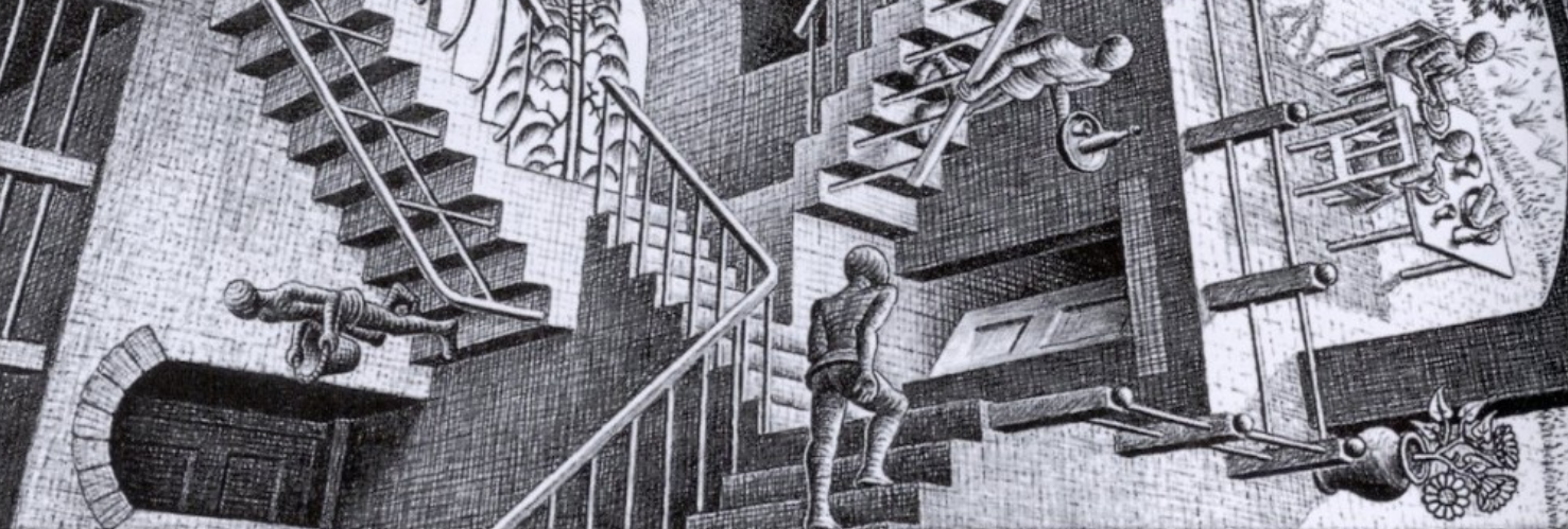
Some of you have probably recognized the above image. That’s “Relativity” one of the most famous lithograph of the artist Maurits Cornelis Escher. In the Relativity world there is the intersection of multiple orthogonal sources of gravity. There are various stairways, and each stairway can be used to move between two different gravity sources. Another interesting Escher’s lithograph is “Ascending and Descending”, where two lines of anonymous men appear over an impossible staircase, one line ascending while the other descends, in a sort of ritual. Escher was inspired by the work of the psychiatrist Lionel Penrose, the father of the physicist Roger Penrose, who was working on the model of an impossible staircase, today known as Penrose stairs. The illusion was published by Lionel and Roger in 1958 as a scientific article “Impossible objects: A special type of visual illusion”. Escher discovered Penroses’ work in 1959 and, fascinated by the illusion, released the lithograph one year later. Now, here comes the mind twist. Roger Penrose (the son of Lionel) was introduced to Escher’s work in 1954, during a conference, and impressed by the artist drawings decided to realise one by his own. After multiple attempts Roger came out with the Penrose triangle. Rogers showed the triangle to his father Lionel who produced some variants, including the Penrose stairs. So the work of Escher could not be possible without the contribution of the Penroses, and viceversa. I find this loop between Escher and the Penroses fascinating, especially because connected with a loopy staircase.

The Bayes stairs

Taking inspiration from the Penrose stairs I coined the term Bayes stairs to describe the different levels of inference one can manage in a Bayesian hierarchical model. Like the Penrose stairs the Bayes stairs bend backward in a recursive twist (more on this in the last step). The Bayes stairs have five steps:

1. Maximum Likelihood (ML)
2. Maximum a Posteriori (MAP)
3. Maximum Likelihood type II (ML-II)
4. Maximum a Posteriori type II (MAP-II)
5. Fully Bayesian treatment

I will show you how climbing the stairs allows us to get closer and closer to a fully Bayesian treatment, just to find ourselves at the very first step once we reach the top of the staircase. Having in mind the Bayes stairs is a useful trick to remember all the options available in Bayesian analysis. Moreover, the stairs can be used during an empirical approach as guidelines. Roughly speaking, the staircase is built such that “more integrals one performs, the more Bayesian one becomes” (Murphy, 2012). Reaching higher steps requires a major effort but also gives a larger payoff.

This post is mainly based on Chapters 5.5 and 5.6 of the book “Machine learning: a probabilistic perspective” by Murphy, and Chapters 5.5 and 5.6 of the book “Deep Learning” by Goodfellow et al. (yes, there is a loop even in the books chapters). Additional resources are reported at the end of the post.

Prerequisites for a good understanding of the post are basic concepts of probability theory and statistics. For instance, I assume you are familiar with random variables, marginal and conditional distributions, Bayes’s rule, likelihood, and Gaussian distributions.

Step 1: Maximum Likelihood (ML)

Let’s consider a simple probabilistic graphical model such as \(\theta \rightarrow x\), where \(\theta\) are parameters representing our model (it can be a scalar or a vector) and \(\mathcal{D} = \{x_n\}_{n=1}^{N}\) is a dataset of \(N\) samples drawn independently from an unknown data-generating distribution \(p(\mathcal{D})\). Our goal is to approximate \(p(\mathcal{D})\) through \(q(\mathcal{D} \vert \theta)\), meaning that we aim at minimizing the Kullback-Leibler divergence (KL) between the two distributions. Abusing the notation for the sake of clarity we write:

\[D_{\mathrm{KL}}(p(\mathcal{D}) \| q(\mathcal{D} \vert \theta))=\int_{-\infty}^{\infty} p(\mathcal{D}) \log \left(\frac{p(\mathcal{D})}{q(\mathcal{D} \vert \theta)}\right) d \mathcal{D}.\]

We can notice that \(p(\mathcal{D})\) is not function of the model parameters \(\theta\), meaning that we only need to consider \(q(\mathcal{D} \vert \theta)\) to minimize \(D_{\mathrm{KL}}\), and since \(q(\mathcal{D} \vert \theta)\) appears in the denominator it means we have to maximize it.

What we came up with, following this reasoning, is a procedure known as Maximum Likelihood (ML) estimation. The objective of ML is to find

\[\hat{\theta}_{\text{ML}} = \text{argmax}_{\theta} \ q(\mathcal{D} \vert \theta).\]

This is generally done by taking the derivative of the log likelihood \(\log q(\mathcal{D} \vert \theta)\) with respect to \(\theta\) and then maximizing via gradient ascent. Note that in ML we are doing a point estimate of the parameters \(\theta\).

The ML estimator can be easily adapted to deal with datasets \(\mathcal{D} = \{(x_n,y_n)\}_{n=1}^{N}\) of input-output pairs, and in fact this is the standard assumption in supervised learning. In this case we assume a model \(\theta \rightarrow x \rightarrow y\) where \(x\) predicts \(y\).

Example: let’s suppose that our dataset \(\mathcal{D} = \{(x_n,y_n)\}_{n=1}^{N}\) is composed by real valued scalars for both input \(x\) and output \(y\). We are in the supervised regression case. We model the output \(y\) as a Gaussian random variable meaning that \(y \sim \mathcal{N}(\mu, \sigma^2)\), this is a reasonable assumption most of the times since it takes into account uncertainty in the data. Our model can be represented as a function \(\mathcal{F}_{\theta}(x) \rightarrow \hat{y}\) mapping the inputs to some approximated output \(\hat{y}\). For instance, if we want to fit a line on the data (linear regression) then \(\mathcal{F}_{\theta}(x) = mx + b\) with parameters \(\theta = [m,b]\) representing the slope and bias of a straight line. In this particular case the Gaussin on \(y\) has mean given by \(\mu = \mathcal{F}_{\theta}(x) = \hat{y}\), leading to the following objective

\[\hat{\theta}_{\text{ML}} = \text{argmax}_{\theta} \ \prod_n p(y_n \vert x_n, \theta) = \text{argmax}_{\theta} \ \prod_n \frac{1}{\sqrt{2 \sigma^2 \pi}} \ \exp \Bigg(-\frac{(y_n - \mathcal{F}_{\theta}(x_n) )^2}{2 \sigma^{2}} \Bigg),\]

where I replaced the likelihood \(p(y \vert x, \theta)\) with the Gaussian distribution \(\mathcal{N}(y \vert \mu=\mathcal{F}_{\theta}(x), \sigma^2)\). In ML we are maximizing this expression, meaning that the normalization constant can be removed. Moreover, taking the logarithm (that cancels out with the exponential and turns products into sums) and considering the variance to be constant and equal to \(\sigma^2=1\), we end up with

\[\hat{\theta}_{\text{ML}} = \text{argmax}_{\theta} \ -\frac{1}{N} \sum_n (y_n - \mathcal{F}_{\theta}(x_n))^2.\]

This is equivalent to the negative Mean Squared Error (MSE) between the data and the model prediction. Maximizing this quantity correspond to minimizing the MSE. Note that, if instead of a linear regressor we were using a neural network to model \(\mathcal{F}_{\theta}(x)\) the results would not change, since backpropagation over the MSE loss has exactly the same meaning.

Problems with ML: for long time ML has been the workhorse of machine learning. For instance, we are implicitly using ML every time we are doing supervised training of a neural network. However, ML is prone to overfitting. A huge model, with millions of parameters, will fit the data almost perfectly, resulting in a very high log likelihood. This means that ML tends to favor complex models against simple ones. A way to attenuate this issue is to introduce a regularization term, this is what we are going to do in the next step…

Step 2: Maximum a Posteriori (MAP)

If our goal is to get the point estimate of an unknown real valued quantity, what we can do is to compute the mean, median or mode of the posterior. Those statistics can be good descriptors of the unknown value. Among those quantities, the posterior mode is the most popular choice because finding the mode reduces to finding the maximum, a common optimization problem. This particular choice is called Maximum a Posteriori (MAP).

In order to move forward to the second step, we need two prerequisites. (i) We have to define a suitable prior distribution parameterized by \(\theta\) (we are still considering the case \(\theta \rightarrow \mathcal{D}\)). A smart choice is a conjugate prior from the exponential family, that will help us with the second prerequisite. (ii) We need an analytical expression for the posterior distribution \(p(\boldsymbol{\theta} \vert \mathcal{D})\) (since we will need to estimate its derivative). When the two prerequisites are satisfied, MAP consists in maximizing the posterior with respect to the parameters, where the posterior is obtained via Bayes’ rule:

\[p(\boldsymbol{\theta} | \mathcal{D}) = \frac{p(\mathcal{D} | \boldsymbol{\theta}) p(\boldsymbol{\theta})}{p(\mathcal{D})}.\]

Since we are interested in finding the mode of the posterior, and the mode does not change before and after normalization, we can get rid of the denominator and just consider the numerator:

\[p(\boldsymbol{\theta} | \mathcal{D}) \propto p(\mathcal{D} | \boldsymbol{\theta}) p(\boldsymbol{\theta}).\]

That’s the final expression we were looking for. Our goal now is to find \(\hat{\theta}\) the value of \(\theta\) that maximize the objective, here defined as:

\[\hat{\theta}_{\text{MAP}} = \text{argmax}_{\theta} \ p(\mathcal{D} | \boldsymbol{\theta}) p(\boldsymbol{\theta}).\]

If you compare the MAP objective and the objective used in ML (see step 1), you will notice that here we are doing the same thing but we are weighting the likelihood by the prior over parameters \(p(\boldsymbol{\theta})\). The effect of adding the prior is to shift the probability mass towards regions of the parameter space that are preferred a priori. Note that if we trivially assume an uniform prior over \(p(\boldsymbol{\theta})\) we fall back to step 1, since the constant term would cancel out and only the likelihood would really matter. Another advantage of using the prior is its regularization effect, which was missing in setp 1. The prior is a constraint over the parameters and in gradient based learning it forces the weights to be updated in specific directions.

Example: let’s continue the example given in the previous section, and let’s suppose that we want to impose a prior distribution over the parameters \(\theta\) of our generic model \(\mathcal{F}_{\theta}\). It would be silly to use an uniform prior, because this is equivalent to ML (previous step). Our likelihood is a Gaussian distribution, therefore we can be smart and use another Gaussian as prior. This will ensure conjugacy if \(\mathcal{F}_{\theta}\) is in an appropriate form. A good choice is a Gaussian with zero mean and variance \(\tau^2\)

\[p(\theta) = \prod_i \mathcal{N}(\theta_i \vert 0, \tau^2) = \prod_i \frac{1}{\sqrt{2 \tau^2 \pi}} \ \exp \Bigg(-\frac{(\theta_i - 0 )^2}{2 \tau^{2}} \Bigg),\]

were we have assumed that \(\theta\) is a vector. If we now apply the same considerations of the previous step (removing the normalization constant, taking the logarithm) we end up with

\[p(\theta) \propto -\frac{\lambda}{2} ||\theta||_{2}^{2},\]

where \(\lambda\) is just the precision (reciprocal of the variance), and we have taken the norm of the vector \(\theta\) (since the logarithm turns the product into a sum over its components). Now recall that MAP consists in finding the mode of the posterior, where the posterior is given by the likelihood times the prior

\[\hat{\theta}_{\text{MAP}} = \text{argmax}_{\theta} \log p(y \vert x, \theta) p(\theta) = \text{argmax}_{\theta} \ -\frac{1}{N} \sum_n \underbrace{(y_n - \mathcal{F}_{\theta}(x_n))^2}_{\text{data-fit}} - \underbrace{\frac{\lambda}{2} ||\theta||_{2}^{2}}_{\text{penalty}}.\]

The above expression can be decomposed in a data-fit (likelihood) and a penalty (prior) term. The penalty in this case is just an \(l_2\) regularizer also known as Tikhonov regularization or ridge regression. In general when a model is overfitting there are many large positive and negative values in \(\theta\). The regularization term encourages those parameters to be small (close to zero), resulting in a smoother approximation, by using a Gaussian prior with zero mean. Note that if we assign a constant value to \(\lambda\) we can tune the strength of the regularization term making the underlying Gaussian distribution more or lees peaked around the mean.

Changing the Gaussian prior into a Laplace prior (or double-exponential prior) we are instead imposing an \(l_1\) penalty, also known as Lasso regularization. This prior is sharply peaked at the origin and it strongly moves the parameters toward zero.

Problems with MAP: we said that MAP corresponds to a point estimate of the posterior mode. It turns out that the mode is usually quite untypical of the distribution (unlike the mean or median that take the volume of the distribution into account), and this is why MAP can still give a rather poor approximation of the parameters. Another problem with MAP is that the prior can sometimes be an arbitrary choice left to the designer and this may influence the posterior in the low-data regime. As we said, using a uniform prior is pointless since we revert to an ML estimate.

Step 3: Maximum Likelihood type II (ML-II)

Step 3 is known as an ML-II procedure since it corresponds to maximum likelihood but at a higher level. To be more precise, we are now considering a probabilistic graphical model with two levels \(\eta \rightarrow \theta \rightarrow \mathcal{D}\), where \(\eta\) are latent variables representing a hyperprior over the prior. This may sound confusing but if you think about that, it makes sense to model the parameter of our prior as another probability distribution instead of relying on a point estimate. This is an example of a hierarchical (or multi-level) Bayesian model. In order to access the third step, it is necessary to compute the posterior on multiple levels of latent variables.

In literature ML-II is also known as Empirical Bayes, since the hyperprior distribution is estimated from the data, meaning that the parameters at the highest level of the hierarchy are set to their most likely values, instead of being integrated out. Note that this assumption violates the principle that the prior should be chosen in advance, independently of the data, as needed in a rigorous Bayesian treatment. This is the price to pay at step 3, for having a computationally cheap approximation.

The main difference with respect to the previous steps is that here the objective is to focus on the set of parameters \(\eta\) used to model the hyperprior. The strategy we use to achieve this objective is to analytically marginalize out \(\boldsymbol{\theta}\), leaving us with the simpler problem of just computing \(p(\eta \vert \mathcal{D})\):

\[\hat{\boldsymbol{\eta}}_{\text{ML-II}}=\operatorname{argmax}_{\boldsymbol{\eta}} \int p(\mathcal{D} | \boldsymbol{\theta}) p(\boldsymbol{\theta} | \boldsymbol{\eta}) d \boldsymbol{\theta}.\]

The above expression is also known as marginal distribution. Marginalizing out \(\theta\) is not always possible, for this reason we have to be clever and use conjugate priors when appropriate. Once this has been done we are left with finding \(\hat{\eta}\), at step 3 this is done using ML. As in step 1 we simply take the derivative with respect to \(\eta\) and then we maximize via gradient ascent.

Problems with ML-II: type II can be considered an improvement over type I. For instance when both the prior and the likelihood are Gaussian distributions, the empirical Bayes estimators (e.g. the James-Stein estimator) dominate the simpler maximum likelihood estimator in terms of quadratic loss and at the same time provide an artifice to avoid the drawback of a fully Bayesian treatment. As pointed out by Carlin and Louis, the empirical Bayes “offers a way to dangle one’s legs in the Bayesian water without having to jump completely into the pool” (Carlin and Louis, 2000). However, even if type II can be considered an improvement, we are still into an ill-formed Bayesian setting. In this regard, I agree with Dempster in saying that an empirical Bayesian is someone who “breaks the Bayesian egg but then declines to enjoy the Bayesian omelette” (Dempster, 1983).

Step 4: Maximum a Posteriori type II (MAP-II)

Level 4 is known as an MAP-II procedure because it corresponds to applying MAP at the higher hyperprior level. Similarly to MAP (see step 2) we need (i) to define a proper hyperprior distribution over \(\eta\), and (ii) to have an analytical form for the posterior over \(\eta\). Additionally, we also need to analytically marginalize out \(\boldsymbol{\theta}\):

\[\hat{\boldsymbol{\eta}}_{\text{MAP-II}}=\operatorname{argmax}_{\boldsymbol{\eta}} \int p(\mathcal{D} | \boldsymbol{\theta}) p(\boldsymbol{\theta} | \boldsymbol{\eta}) p(\boldsymbol{\eta}) d \boldsymbol{\theta}.\]

What are exactly the parameters \(\eta\)? Well, it depends from the type of distribution associated to the prior. If our prior is a Gaussian distribution we need to set an hyperprior for the mean and variance of such a Gaussian. Moreover, we also need the posterior over the hyperprior in order to apply MAP-II. To get an analytical posterior it is necessary to use a conjugate hyperprior.

Where does the strength of type II inference come from? Hierarchies exist in many datasets and modelling them appropriately adds statistical power. The strength comes from borrowing statistical strength from the experience of others. This has been clearly pointed out for the James–Stein estimator, where given case 1, it is possible to learn from the experience of the other \(N-1\) cases (see Efron, 2012, Chapter 1). The exact meaning of this passage will become evident in the example at the end of the post.

Step 5: Fully Bayesian

We are on top at the last step. Over here it is possible to perform inference at any level, and to estimate all the posterior distributions encountered so far. If you are thinking that this is too good to be true then you are right. A fully Bayesian treatment for non-trivial hierarchical models is only possible through sampling methods, such as Markov Chain Monte Carlo (MCMC). This is computationally expensive and it requires some experience in tuning the parameters of the sampler (e.g. warmup period).

When to go for a fully Bayesian treatment? Hard to say, it depends from the problem at hand and the data available. We need a fully Bayesian treatment whenever we are not happy with a point estimate, in this case a fully Bayesian treatment would unlock the posterior.

During the years have been proposed some methods that represent a compromise between a point estimate and a fully Bayesian treatment, such as the Laplace approximation, expectation propagation, and variational approximation. As the names suggest, all these methods perform an approximation of the posterior distribution. Whether this approximation is good or no depends from the shape of the posterior and the distribution used to approximate it. For instance, if the posterior is multi-modal and we are using a Gaussian to approximate it, then our approximation risks to be rather poor.

Note that step 5 can be considered as step 0, like in Penrose stairs and Escher’s Ascending and Descending. In fact, we can decide to directly go for a fully Bayesian treatment from the very beginning, without having to climb the staircase at all. However, very often only an empirical approach will show which is the right method to use and this requires climbing the Bayes stairs more than once (hopefully not in an eternal loop).

Example: robotic arms

The startup Reactive-Bots is producing and selling robotic arms. Their latest product is a complex 6-dof cordless arm which can be used both in industry and academia for manufacturing and research. The distinctive characteristic of the new model is the use of an internal battery which allows deploying the arm in situations where a power socket is not available.

You have been recently hired in the R&D department and you have been asked to estimate the average power consumption of the arm. Your estimate is particularly important because it will be used to define a software failsafe trigger that protects the battery against an overload. From now on we will be concerned with the problem of finding the mean power consumption, assuming that the variance is given.

Step 1: from a preliminary analysis you notice that there are large power fluctuations due to external and internal factors (e.g. workload, room temperature, etc) therefore to get a good estimate you decide to record the power for a period of several hours in laboratory conditions, and then estimate the mean over \(N\) different arms.

Let’s formalize the problem defining a dataset \(\mathcal{D} = \{x_n\}_{n=1}^{N}\) with \(x_n \in \mathbb{R}\) and no labels (unsupervised). The shape of the underlying data generating distribution is unknown, but common sense suggest it may have a bell-like shape, we go for a Gaussian likelihood. The use of a Gaussian distribution is particularly well suited for the problem at hand, because if you get the mean and the standard deviation right, it will be possible to easily detect abnormal spikes and trigger the failsafe. More formally, let’s define \(\mathcal{F}_{\theta}\) as a Gaussian distribution with parameters \(\theta = [ \mu, \sigma^2 ]\) representing the mean and variance.

Now, we want to use \(\mathcal{F}_{\theta}\) to approximate the data generating distribution. At the first step of the Bayes stairs this can be done through ML estimation. The parameter we need to estimate is the mean \(\mu\) (as said above we are not concerned about the variance), this has a closed form expression that can be easily obtained taking the logarithm of the Gaussian and then the derivative

\[\hat{\mu}_{\text{ML}}=\frac{1}{N} \sum_{n=1}^{N} x_{n}.\]

It turns out that ML estimation of a Gaussian just consists in the estimation of the empirical mean over the \(N\) data points.

Step 2: there is another information we should take into account in our estimation. The battery has an optimal functional range, respecting this range maximizes the operational life span. Following this line of thoughts you consult the datasheet of the battery and notice that the manufacturer has reported the optimal average and standard deviation that guarantees maximal life span, this can be used as a prior.

To ensure conjugacy the prior over the mean is defined as a Gaussian with parameters \(\theta_0 = [ \mu_0, \sigma_{0}^{2} ]\) representing the mean and variance taken from the datasheet. The posterior is given by the product between the prior and the likelihood

\[p(\mu) p(x \vert \mu)=\frac{1}{\sqrt{2 \pi} \sigma_{0}} \exp \left(-\frac{(\mu-\mu_{0})^{2}}{2\sigma_{0}^2} \right) \prod_{n=1}^{N} \frac{1}{\sqrt{2 \pi} \sigma} \exp \left(-\frac{(x_{n}-\mu)^{2}}{2\sigma^2}\right).\]

Using a few tricks (e.g. completing the square) we can get the following form for posterior mean

\[\hat{\mu}_{\text{MAP}}=\frac{\sigma_{0}^{2} N}{\sigma_{0}^{2} N+\sigma^{2}}\left(\frac{1}{N} \sum_{n=1}^{N} x_{n}\right)+\frac{\sigma^{2}}{\sigma_{0}^{2} N+\sigma^{2}} \mu_{0}.\]

The last term shows that MAP estimation of the mean in the Gaussian model is just a linear interpolation between the sample mean (the term in parentheses) and the prior mean \(\mu_{0}\), both of them weighted by their variances.

Step 3: Reactive-Bots has finished the design and test of the arms and went on with production and selling. For the second version of the arm there are important updates planned, those are based on the feedback of the customers. In particular it turned out that a single failsafe threshold is not so useful in practice and that it would be ideal to adapt it to the use case. For instance, some customers are using the arms for the fine grained pick and place of small objects, whereas others are using the arms for heavyweight manufacturing. It seems reasonable to decrease the failsafe threshold for the former (to identify anomalies in the low-power regime) and increase it for the latter (to avoid sudden drops in the high-power regime).

Even though you have acquired data from \(N\) different arms in controlled lab conditions, there is still a wide range of real-world scenarios you have not considered. The arm performance in those settings is not clear to you. It is necessary to investigate the problem acquiring the telemetry from each customer, then find a new estimate of the average power in each application and start working on the upgraded version of the arm controller.

To formalize the problem we suppose that the dataset \(\mathcal{D}\) is divided in chunks such that \(\mathcal{D} = \{\mathcal{D}_m\}_{m=1}^{M}\) and that each chunk represents a customer, with the data samples \(\mathcal{D}_m = \{x_n\}_{n=1}^{N_m}\) being the power measurements acquired via telemetry. Note that each customer bought a different number of arms, indicated as \(N_m\). As before we assume that the data generating distribution can be modelled with a Gaussian \(\mathcal{N}(x \vert \mu_m, \sigma^{2}) \ \forall x \in \mathcal{D}_m\). In other words, the parametric function \(\mathcal{F}_{\theta}\) is here a Gaussian, with \(\theta = [ \mu_m, \sigma^2 ]\).

One way to go would be to use a simple ML or MAP approach (1st and 2nd step of the stairs) to estimate the average power for each customer. However, there are some customers that just bought a few arms, and others that bought thousands of them. While it is easy to find the average power for the data-rich groups, it is significantly more difficult for data-poor groups. It would be great if we could somehow take into account the samples of data-rich groups when estimating the posterior distribution of data-poor groups. It turns out we can do that if we add another level of inference in our probabilistic model.

We assume that the parameters describing the Gaussian associated to each dataset have been drawn from a common hyper distribution. In our particular case we assume this distribution to be another Gaussian. Note that this is exactly the formulation we used to describe the hyperprior in step 3 of the Bayes stairs. Since we have a Gaussian describing each dataset and a Gaussian as hyperprior, this probabilistic model is often called Gaussian-Gaussian and it is here defined as \(\eta \rightarrow \theta_{m=1}^{M} \rightarrow x_{n=1}^{N_m}\), with \(\eta=[\nu, \tau^2]\) being the mean and variance of the hyperprior. Given these assumptions we can estimate the joint distribution as follows:

\[p\left(\mu, \mathcal{D} \vert \hat{\eta}, \sigma^{2}\right)=\prod_{m=1}^{M} \mathcal{N}\left(\mu_{m} | \hat{\nu}, \hat{\tau}^{2}\right) \prod_{n=1}^{N_{m}} \mathcal{N}\left(x_{n m} | \mu_{m}, \sigma^{2}\right).\]

We have taken the point estimate of the hyperprior parameters \(\hat{\eta}\) since we are in the ML-II setting. Now, we can simplify the above expression considering that the \(N_m\) Gaussian measurements in group \(m\) are equivalent to one measurement with mean and variance given by

\[\bar{x}_m = \frac{1}{N_m} \sum_{n=1}^{N_m} x_{nm}, \ \ \sigma^{2}_{m} = \frac{\sigma^2}{N_m}.\]

The variance shrinks with the number of observations, since we get more and more confident about the true value. We now want to find the posterior distribution of the mean for a specific group \(m\), this can be done as follows:

\[p(\mu_m, \vert \hat{\eta}, \mathcal{D}) = \mathcal{N}\left(\mu_m | \hat{B}_{m} \hat{\nu}+\left(1-\hat{B}_{m}\right) \bar{x}_{m},\left(1-\hat{B}_{m}\right) \sigma_{m}^{2}\right), \ \ \text{with} \ \ \hat{B}_{m} = \frac{\sigma_{m}^{2}}{\sigma_{m}^{2}+\hat{\tau}^{2}}.\]

It is worth spending some words to analyze the above expression in particular the shrinkage factor \(\hat{B}_{m} \in [0,1]\). This factor controls the degree of shrinkage towards the hyperprior mean \(\hat{\nu}\). If the sample size \(N_m\) for group \(m\) is large, then \(\sigma^{2}_{m}\) will be small in comparison to \(\hat{\tau}^{2}\) reducing \(\hat{B}_{m}\). When \(\hat{B}_{m}\) is small (data-rich groups) then \(\hat{\nu}\) is small and \(\bar{x}_{m}\) is large, meaning that we put more weight on the actual measurements respect to the hyperprior mean. When \(\hat{B}_{m}\) is large instead (data-poor groups), we get the opposite effect with the hyperprior mean having more weight over the posterior.

This is exactly what we wanted in our example, data-poor groups will have a small shrinkage factor with the hyperprior counting more. However, we also said that we wanted to take advantage of data-rich groups in the posterior of data-poor groups. How is this obtained? This is automatically done when we perform ML-II on the hyperprior parameters. Taking the derivative with respect to \(\hat{\nu}\) we get that the ML estimate corresponds to

\[\hat{\nu} = \frac{1}{M} \sum_{m=1}^{M} \bar{x}_m.\]

What does this expression is telling us? The mean of the hyperprior is given by the average over all samples, therefore groups with more samples will have a larger effect on \(\hat{\nu}\) influencing the posterior of data-poor groups. Note that if we assume \(\sigma_m = \sigma\) for all groups then we just have the James-Stein estimator.

Step 4: if we have good reasons to assume that the hyperprior mean is close to a specific value then we can define a Gaussian prior over \(\eta\) embedding such an assumption (yes, that would be a prior over the hyperprior). This has the same regularization effect discussed for MAP type I at step 2, moving the average \(\hat{\nu}\) toward the prior mean. In particular we would end up with a linear interpolation between two terms: (i) the prior mean, and (ii) the sample mean, both of them weighted by their respective variances. Also in this case assuming a uniform prior instead of a Gaussian one, we fall back to step 3 since we would be doing just ML-II. I will skip a detailed derivation here, which is left as an exercise for the reader.

Step 5: at the beginning of this example we made the simplifying assumption that the posterior distribution over the power consumption of the robotic arms could be modelled relatively well by a Gaussian distribution. However, let’s remember that the Gaussian may be a rather poor approximation if the posterior is multimodal. Another reason why we choose a Gaussian is that there is a conjugate prior we can use to get the posterior in a closed form. Moving toward other distributions we can lose this helpful property ending up with an intractable posterior.

Is there a way to avoid this oversimplification? Well yes, that is exactly what you can do in the last step of the Bayes stairs. Methods such as MCMC are distribution agnostic, meaning that you can go for a full Bayesian treatment without worrying to much about the shape of the posterior. However, this incur in a significant computational cost and it also requires a certain experience in tuning the hyperparameters of the sampler. A detailed discussion of this step is out of scope and it would require another blog post.

Conclusions

In this post I gave you an overview of Bayesian hierarchical models using the metaphor of the Bayes stairs. Climbing the stairs corresponds to performing Bayesian inference at different levels. It is necessary to have a deep insight into the problem at hand in order to understand which step should be considered the final one. Most of the time this requires an empirical approach, moving up and down, until the optimal solution is reached.

That’s all folks! If you liked the post please share it with your network and give me some feedback in the comment section below. I send you my greetings with the hope that you enjoyed climbing the Bayes stairs.

References

Carlin, B. P., & Louis, T. A. (2000). Empirical Bayes: Past, present and future. Journal of the American Statistical Association, 95(452), 1286-1289.

Dempster A.P. (1983). Parametric empirical Bayes inference: theory and applications. Journal of the American statistical Association.

Efron, B. (2012). Large-scale inference: empirical Bayes methods for estimation, testing, and prediction (Vol. 1). Cambridge University Press.

Goodfellow, I., Bengio, Y., & Courville, A. (2016). Deep learning. MIT press.

Murphy, K. P. (2012). Machine learning: a probabilistic perspective. MIT press.